

Recently, I was side-tracked by a stumble into the Wikipedia article on fractional Fourier transforms. I found it interesting, because normally I think of the Fourier transform as an all-or-nothing proposition. I'm either thinking in the frequency domain or in the time domain, not some combination both. What would it even mean to be in a combination of both domains?
Of course there must be some meaning here. The Fourier transform can be represented as a unitary matrix $F$, and unitary matrices have well-defined square roots and cube roots and so forth. For any fractional parameter $s$, there must be some actual matrix $M$ that is a solution to $F^s = M$ . (Actually, we can find an uncountable infinity of such solutions! But we'll be focusing on a "natural" one.)
Now $F^s$ may be a complicated matrix, or maybe not, I don't know. But I started wondering about how expensive it would be, given $s$, to apply this strange $F^s$ operation. As is typical for a function-of-a-matrix question of this kind, the answer is all about the eigenvalues and eigenvectors. In particular, as I was surprised to learn from the wiki article, the Fourier transform's matrix has very convenient eigenvalues.
If you Fourier transform a vector twice, the result is the same vector but with all of the elements (except the first element) in reverse order. Apply the Fourier transform two more times, so a second reversal undoes the first, and you're back to the original vector. This means that $F^4 = I$, i.e. applying the Fourier transform four times is equivalent to doing nothing. Which means that each eigenvalue $\lambda$ of $F$ must satisfy $\lambda^4 = 1$. There are only four solutions to that equation: $\lambda \in \{1, i, -1, -i\}$. So those are the only four eigenvalues of $F$.
The eigenvalue set $\{1, i, -1, -i\}$ is convenient for several reasons. First, it's small. There's only four possibilities. Second, it's closed under multiplication. In other words, the eigenvalues are evenly spaced around the complex unit circle. Third, the set's size is a power of 2. These all happen to be useful when it comes to constructing a short quantum circuit.
The Fractional Quantum Fourier Transform
If you asked me two days ago how gross it would be to make a quantum circuit that applies the square root of a Fourier transform, I would have answered "probably pretty gross". Big complicated operations aren't guaranteed to have nice circuits that apply their square root, so why would you expect there to be a nice circuit for some specific operation? You'd need the operation to just happen to follow some kind of nice pattern... like having an extremely convenient set of eigenvalues.
A small evenly-spaced set of eigenvalues is great because it means phase estimation can pull apart the parts of the vector corresponding to each eigenvalue. This gives you a way to index into each part, and phase them independently, before putting them back together. The eigenvalue set $\{1, i, -1, -i\}$ is perfect for phase estimation, because it's exactly the set of eigenvalues that a 2-qubit phase estimation will pull out without error.
Apply a 2-qubit phase estimation to the QFT, and you get this circuit:
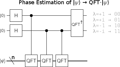
The above circuit is correct, but unnecessarily expensive. We know that two applications of the QFT to a register is equivalent to negating the register's value (i.e. reversing the order of all states except $|0\rangle$). Instead of using two QFTs, we can use the fact that $\lnot x + 1 = -x-1 + 1 = -x$. It's much cheaper to NOT-and-increment than it is to apply two QFTs:
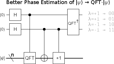
So what does this circuit do? Well, if the target register (the one we're hitting with a QFT, NOT, and increment) is storing an eigenvector of the Fourier transform, then the controls, Hadamards, and inverse-QFT will cause that eigenvector's eigenvalue to "kick back" into the phase estimation register. In effect we have performed a temporary measurement (namely "which eigenspace is the target register in?"). The result of that "measurement" is being held in the phase estimation register. Of course we don't want to actually measure. In practice the input will be a superposition of multiple eigenvectors, and so the phase estimation register will end up storing an entangled superposition of values. We don't want our fractional QFT causing decoherence, so we don't want to collapse that superposition.
As an example, suppose $|v\rangle$ is an eigenvector of the QFT with eigenvalue $-i$, and $|w\rangle$ is an eigenvector with eigenvalue $-1$. Applying the phase estimation circuit to the state $|00\rangle \otimes (|v\rangle + |w\rangle)$ will produce the entangled state $|11\rangle \otimes |v\rangle$ + $|10\rangle \otimes |w\rangle$. Notice that, if we then apply a controlled-Z operation to the phase estimation register, it will negate the $|11\rangle$ part of the state but leave the $|10\rangle$ part alone. But since the $|11\rangle$ part is entangled with the $|v\rangle$ part and the $|10\rangle$ part is entangled with the $|w\rangle$ part, we can instead think of this CZ operation as negating the $|v\rangle$ part while leaving the $|w\rangle$ part alone. The phase estimation register gives us a way to independently phase each eigenvalue's eigenspace!
The amount we want to phase each part by is determined by our goal: to perform a fractional QFT. If we want to perform $QFT^S$, and the normal QFT phases an eigenvector by $p$, then our fractional QFT will phase that eigenvector by $p^s$. Note that $p^s$ often has several solutions. For example, $1+i$ and $-1-i$ are both perfectly valid squares roots of $2i$. We break this ambiguity by arbitrarily representing $p$ as $e^{i \theta}$ with $\theta \in [0, 2 \pi)$, and declaring that $p^s = (e^{i \theta})^s = e^{i s \theta}$.
Because the phase estimation register ends up indexing the eigenvectors as $+1 \rightarrow 00$, $i \rightarrow 01$, $-1 \rightarrow 10$, and $-i \rightarrow 11$, phasing by the correct amount is trivial. We simply apply a phase gradient to the register: hit the low bit with $Z^{s/2}$ and the high bit with $Z^{s}$. This phases $|00\rangle$ by nothing, $|01\rangle$ by $(-1)^{s/2}$, $|10\rangle$ by $(-1)^s$, and $|11\rangle$ by $(-1)^{3s/2}$. The usual QFT is at $s=1$, and the inverse QFT is at $s=-1$.
After we have phased the eigenvectors by the correct amount, we have to put them back together. That is to say, we need to disentangle the phase estimation register from the target register by uncomputing the phase estimation. This gives us the final circuit:
![]()
So it turns out that two applications of the raw QFT, with some ancillae phasing in between, is enough to apply any fractional power of the QFT! (I'm not counting the QFTs on the phase estimation register because they don't scale with the number of target register qubits, and 2-qubit QFTs are trivial.)
I created an example fQFT circuit in my simulator Quirk. It also includes some framing that causes an amplitude display to basically show the operation's matrix cycling through $I$, the FFT, the negation-permutation, and the inverse FFT.
This apply-fractional-power-by-phasing-the-phase-estimation trick is very general. It works on any operation amenable to phase estimation. The trick worked on the QFT because the QFT has a nice small evenly-spaced set of eigenvalues, but it also works if you have some way to apply large integer powers of an operation (and a non-zero tolerance for errors). It is very much a tool worth keeping in your toolbox.
A Classical Fast Fractional Fourier Transform
I've mentioned in the past that the simplest QFT circuit is just a direct translation of Cooley-Tukey FFT algorithm into the language of quantum circuits. The translation works the other way, too: given the simple QFT circuit, you can mechanically produce classical code equivalent to the Cooley-Tukey algorithm. The same is true of the fractional QFT circuit we've derived: we can translate it into a fast classical algorithm for fractional Fourier transforms.
Reading our fQFT circuit roughly from left to right, each operation tells us some classical code to add:
$H$ on $|0\rangle$:
Make a copy of the input vector.
Controlled QFT:
Fourier-transform the copy we just made. Note that we want the unitary Fourier transform; the one that preserves the 2-norm. In numpy, you get this by adding
norm='ortho'to the fft call. Otherwise the result will be scaled up by a factor of $\sqrt{N}$ compared to what we want.$H$ on another $|0\rangle$:
Make a copy of each of the two vectors we have (the input and its Fourier transform).
Controlled negation:
Apply the reverse-except-0 permutation to the two copies we just made.
inv-QFT on phase estimation register:
Replace the vectors we have ($a$ and $b$ and $c$ and $d$) with some simple linear combinations thereof ($a+b+c+d$ and $a+ib-c-id$ and $a-b+c-d$ and $a-ib-c+id$).
Phase gradient:
Scale each of our four vectors by an appropriate phase factor.
QFT on phase estimation register:
Replace the vectors we have with some simple linear combinations thereof.
Uncomputation stuff:
Return the first vector. Discard the other three.
With a bit of cleanup, and some after-the-fact interpretation of what the operations mean, I produced the following python code:
import numpy as np

def fast_fractional_fourier_transform(vec, exponent):
    # Compute Fourier transform powers of vec.
    f0 = np.array(vec)
    f1 = np.fft.fft(f0, norm='ortho')
    f2 = negate_permutation(f0)
    f3 = negate_permutation(f1)

    # Derive eigenbasis vectors from vec's Fourier transform powers.
    b0 = f0 + f1 + f2 + f3
    b1 = f0 + 1j*f1 - f2 - 1j*f3
    b2 = f0 - f1 + f2 - f3
    b3 = f0 - 1j*f1 - f2 + 1j*f3
    # Note: vec == (b0 + b1 + b2 + b3) / 4

    # Phase eigenbasis vectors by their eigenvalues raised to the exponent.
    b1 *= 1j**exponent
    b2 *= 1j**(2*exponent)
    b3 *= 1j**(3*exponent)

    # Recombine transformed basis vectors to get transformed vec.
    return (b0 + b1 + b2 + b3) / 4


def negate_permutation(vec):
    """Returns the result of applying an FFT to the given vector twice."""
    head, tail = vec[:1], vec[1:]
    return np.concatenate((head, tail[::-1]))
The amazing thing about this code is that the most expensive step is f1 = np.fft.fft(f0, norm='ortho'), which delegates to the normal fast fourier transform.
We're computing a fractional FFT using just one normal FFT, three vector-scalar multiplications, and a handful of vector-vector additions!
(I'm not counting multiplying by $i$, negating, or dividing by $4$ as vector-scalar multiplications; they can be done with addition.)
As with the fractional QFT circuit, I'm struck by how simple things ended up being. I would have expected a classical fast fractional Fourier transform to be way more complicated than this.
Closing Remarks
Although I did find the presented classical fractional FFT algorithm on my own, it isn't novel. An $O(N \lg N)$ algorithm was published in the year 2000 paper "Closed-Form Discrete Fractional and Affine Fourier Transforms" by Soo-Chang Pei and Jian-Jiun Ding.
The FFT has degenerate eigenvalues, and as a result there's a continuous infinity of possible fractional FFTs. For example, it is perfectly valid to define a fractional FFT that phases orthogonal parts of the same eigenspace in different directions (as long as the phases still sync up when $s$ is an integer). The presented algorithm can be tweaked to use other phase sweeps, but it can't handle the case where vectors that agree on FFT eigenvalue disagree on fractional FFT eigenvalue. In a sense, this means that the algorithm is unable to perform almost all of the possible fractional Fourier transforms! I did try to pick a natural choice for how to sweep the phase factors, but I haven't read enough to know if it's the standard choice or even a good choice.
All those caveats aside, I think the presented algorithm makes a good example of quantum algorithms informing the construction of classical algorithms. Knowing the quantum phase estimation trick produced an $O(N \lg N)$ classical fractional FFT in an afternoon, instead of over a series of papers spanning years.
