This is a followup to a post from last year, about the pre-print 'A linear time quantum algorithm for 3SAT' by Zachary B. Walters.

In that post, I argued that the algorithm doesn't do any quantum work. In the comments, Walters and I went back-and-forth. Since then, Walters has updated the paper three times. I suppose it's time to revisit.

After reading the updated paper, I have the same objections as before:

1. This is actually a classical algorithm in disguise.
2. It runs in exponential time, not linear time.

This time, I'll argue my point by simulating the algorithm with Microsoft's LIQUi|> library.

Walters' Algorithm

Before I jump into simulating the algorithm, I need to explain what the algorithm actually does. Basically, it's a quantum version of the idea "if a clause isn't satisfied, perturb that clause's variables".

The paper defines the relevant gates in Section 4. First, the paper defines a "QOR" gate (note: the "R" gates are rotating around the Y axis):

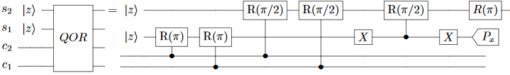
This is supposed to set $s_2$ to $c_1 \lor c_2$, and it does. The problem is $s_1$, which ends up containing the parity of $c_1$ vs $c_2$. The paper recognizes that this is a problem (it will cause unwanted decoherence) but claims that measuring $s_1$ along the X axis can fix the problem. That's simply wrong. The correct fix is to uncompute $s_1$, or avoid creating it in the first place via a doubly-controlled operation.

The paper doubles down on the how-erasure-works misconception when defining the "3OR" gate:

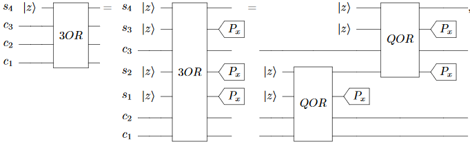
This gate initializes $s_4$ to $c_1 \lor c_2 \lor c_3$, but in the process it exposes $c_1 \oplus c_2$, $c_1 \lor c_2$, and $(c_1 \lor c_2) \oplus c_3$ to the environment via $s_1$, $s_2$, and $s_3$. This is enough to reconstruct all three inputs, so all the qubits are decohered after this gate is applied. Once again the correct fix would be to uncompute or to use multi-controlled gates.

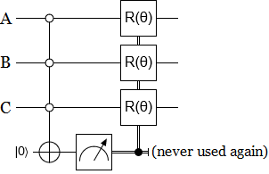
Finally we get to the pièce de résistance, the awesomely-named DECIMATION gate:

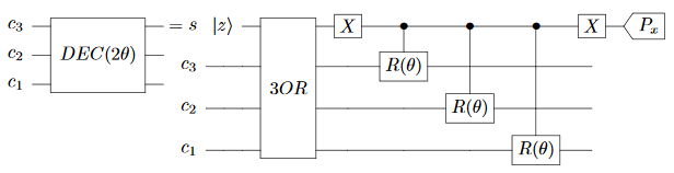
The idea behind this gate is that, when $c_1$ and $c_2$ and $c_3$ fail to meet a clause, they get rotated a bit.

Note that this circuit has yet another attempt to destroy indestructible information by measuring it along a different axis. But this time we can't fix it by adding more controls or by uncomputing, because the values we need to do that no longer commute with the values we have. This is the first major flaw in the paper, I think.

Walters claims that measuring the scratch qubit along a perpendicular axis will fix the problem, and he's simply wrong. However... some phrasing in the paper indicates that the decoherence is actually... desired? The paper often talks about "incoherently transferring" states, for example. So it's hard to say if this is a flaw-in-intent or flaw-in-execution or a flaw-in-explanation or what.

Anyways... here's the whole DE̡͊͠͝CIMATION circuit, expanded in full:

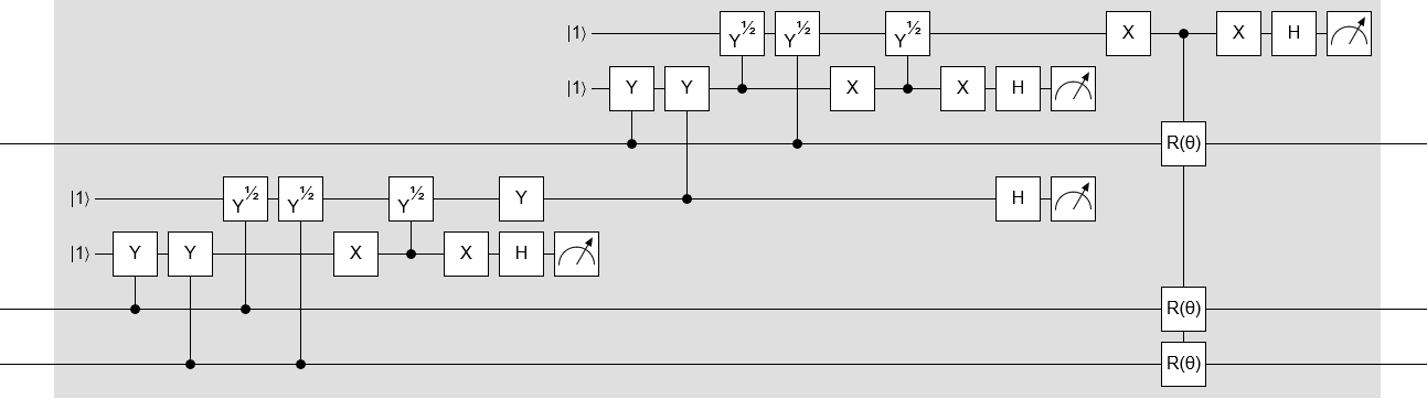
Note that this circuit is specifically for true-or-true-or-true clauses. You have to temporarily invert the inputs to adapt it to other clauses.

The above circuit is kind of daunting. But if you actually pay attention to how the paper describes the operation, and what it's supposed to do, a much simpler DE̡͊͠͝Cͮ̂҉̯͈͕̹̘̱IM̯͍̭̚​̐ATIO̘̝̙ͨ̃ͤ͂̾̆N circuit suggests itself:

Note that this circuit isn't strictly equivalent to Walters' DE̡͊͠͝Cͮ̂҉̯͈͕̹̘̱I̶̷̧̨̱̹̭̯̙̲̝͖ͧ̾ͬͭ̏ͥͮͮ͟͏̮̪̝͍M̯͍̭̚​̐AT̴̨̟̟͙̞̥̫͎̭̑ͩ͌ͯ̿̔̀͝ͅIO̘̝̙ͨ̃ͤ͂̾̆N circuit. It causes a lot less decoherence, for example. Regardless, I think it's much closer to the paper's description of what the gate should do than the circuit that's actually included in the paper.

Because I think this shorter circuit better represents the intent of the paper, I'm torn between whether or not I should use it or the actual circuit from the paper when simulating. On the one hand, any changes I make could be pointed to as the reason the algorithm doesn't work. On the other hand, there's so many gates in Walters' construction that I'm more worried about misplacing one than I am about misinterpreting the intent of the algorithm.

What I'm going to do is compromise a bit. I'm going to use my shorter circuit, but tweaked to do the wrong-axis erasure thing even though I think it's pointless.

Simulation Strategy

My simulation code is available on github, in the repository Strilanc/NP-vs-Quantum-Simulation-Walters-Algorithm.

Generally, the simplest way to show that a 3-SAT algorithm takes exponential time is to just find a problem instance it does poorly on. I think that Walters' algorithm is equivalent to the classical algorithm where you randomly toggle variables in clauses that aren't satisfied, so that's the algorithm I used when looking for difficulties. After some experimentation, I found that there are three basic tricks to making a hard instance:

• Use clauses where only one of the three variables is correct, so that toggling tends to hurt twice as much as it helps.
• Make long chains, where variable N doesn't feel any toggle pressure until variable N-1 is correct.
• Include a reset mechanism, where one wrong variable tends to cause all variables to go wrong.

Here's the F# code I use to construct hard instances. Note that when I say "hard" I just mean "hard for this algorithm", not hard in general. The generated instances are actually very easy: there's always exactly one trivial solution.

let evil3SatInstance varCount =
    let no i = {index = i; target = false}
    let YA i = {index = i; target = true}

    // Seeding. First three variables must be false.
    let seed = [
        Clause(no 0, YA 1, YA 2);
        Clause(no 0, YA 1, no 2);
        Clause(no 0, no 1, YA 2);
        Clause(no 0, no 1, no 2);
        Clause(YA 0, no 1, no 2);
        Clause(YA 0, no 1, YA 2);
        Clause(YA 0, YA 1, no 2);
    ]

    // Chaining. A variable must be false if the two before it are false.
    let chain =
        seq { 0 .. (varCount-4) }
        |> Seq.map (fun i -> Clause(YA(i+1), YA(i+2), no(i+3)))
        |> List.ofSeq

    // Reset mechanism.
    // 1. Every variable tends to become true if a,b is broken
    // 2. Any true variable tends to break a,b
    // 3. These tendencies are statistically stronger than the tendency to fix any one breakage
    let reset =
        seq { 0 .. (varCount-4) }
        |> Seq.map (fun i ->
            [
                Clause(no(0), no(1), YA(i+3));
                Clause(no(0), YA(1), YA(i+3));
                Clause(YA(0), no(1), YA(i+3));
            ])
        |> Seq.concat
        |> List.ofSeq

    List.concat [seed; chain; reset]

And here's the 27 clauses that make up the 8-variable problem I'll actually be testing on:

!a or b or c
!a or b or !c
!a or !b or c
!a or !b or !c
a or !b or !c
a or !b or c
a or b or !c
b or c or !d
c or d or !e
d or e or !f
e or f or !g
f or g or !h
!a or !b or d
!a or b or d
a or !b or d
!a or !b or e
!a or b or e
a or !b or e
!a or !b or f
!a or b or f
a or !b or f
!a or !b or g
!a or b or g
a or !b or g
!a or !b or h
!a or b or h
a or !b or h

(Originally I planned to do a 16 variable problem, but the simulation was a couple order of magnitudes slower than I expected ahead of time so I dropped back to 8.)

Finally, here's my implementation of Walters' algorithm:

// Perturb-if-not-satisfied-er.
let decimate (power1:int) (power2:int) (qs:Qubits) (Clause(A, B, C)) =
    let CCCNot = Operations.Cgate Operations.CCNOT
    let CPerturb = Operations.Cgate (fun reg ->
        // Turn the Z^(2^-power1 + 2^-power2) gate into an X rotation via surrounding Hadamards
        Operations.H reg
        Operations.R -power1 reg
        Operations.R -power2 reg
        Operations.H reg)

    let scratch = qs.[qs.Length-1]
    let qA = qs.[A.index]
    let qB = qs.[B.index]
    let qC = qs.[C.index]

    // '3-OR' the three variables into the scratch qubit
    if A.target then Operations.X [qA]
    if B.target then Operations.X [qB]
    if C.target then Operations.X [qC]
    CCCNot [qA; qB; qC; scratch]
    if A.target then Operations.X [qA]
    if B.target then Operations.X [qB]
    if C.target then Operations.X [qC]

    // When clause isn't sarget = b perturb the involved qubits
    CPerturb [scratch; qA]
    CPerturb [scratch; qB]
    CPerturb [scratch; qC]

    // Discard the scratch qubit
    Operations.H [scratch] // <-- not necessary
    Operations.M [scratch] // <-- could be done right after the CCCNot
    Operations.Reset Bit.Zero [scratch]

// Iterated per-clause perturb-if-not-satisfied-er.
let waltersDecimationAlgorithm clauses steps (vars:Qubits) =
    // Init into uniform superposition of all assignments (skipping scratch bit).
    for var in vars.[0..vars.Length-2] do
        Operations.H [var]

    // Decimate every clause again and again until we hit the given number of repetitions.
    let rand = new Random()
    for i in 1..steps do
        // The decimation power starts high (90 deg) and scales down slowly over time.
        let power1 = -3

        for clause in clauses do
            let power2 = if rand.NextDouble() < 0.5 then -2 else -3
            decimate power1 power2 vars clause

        // Debug output.
        let probs = String.Join(" ", (vars |> List.map (fun e -> String.Format("{0:0}%", e.Prob1*100.0).PadLeft(4))))
        let degs1 = 360.0*(Math.Pow(2.0, float(power1)) + Math.Pow(2.0, float(power1) + float(-1)))
        let degs2 = 360.0*(Math.Pow(2.0, float(power1)) + Math.Pow(2.0, float(power1) + float(-2)))
        printf "Iter %d, Angles %0.1f vs %0.1f degs, Qubit Probs %s\n" i degs1 degs2 probs

    // Measure result.
    for var in vars do
        Operations.M [var]

Note that I did have to make a few guesses when implementing Walters' algorithm. For example, the paper says to randomly vary the perturbation angle between two values for every clause and that the number of iterations needed should be constant (regardless of problem size). It doesn't give specific angles to use, or say exactly how big "constant" is, so I just picked values myself.

Anyways, enough hedging. Let's try it!

Simulation Results

Here's a recording of a typical run of Walters' algorithm on the 8-qubit problem, stopping after 1000 iterations. Because we're using a simulator, we can see intermediate probabilities. The only valid solution is "all qubits off", so we want all the probability-of-ON columns to be showing 0%.

Watch closely:

I want you to focus on the second column from the right. In particular, notice how it sporadically jumps downward but then gets pulled back to 100%. Eventually, around iteration 900, it makes a big enough jump to escape and reach the solution state.

If Walters is right when he claims that the algorithm should quickly decay to a satisfying solution, what keeps pulling that qubit back to 100%-ON? The paper describes the algorithm as a sort of gentle flow through the graph of states, accumulating at the solution. From that you would expect the probabilities to gradually transition from 50% to the target values, possibly with a few detours, as wrong states lose amplitude. But the simulation shows that actually the state is being jerked around and tossed into the later-qubits-are-mostly-ON bin again and again.

When I run the classical variant of this algorithm, where you store a single state and randomly toggle variables in unsatisfied clauses, the same behavior shows up. The system gets stuck in states where the later variables are almost always true, and the reset mechanism keeps breaking the gradual chaining towards a solution. The 'jumps' are just chains that made it unusually far before being reset.

Both the classical algorithm and Walters' algorithm take, typically, a couple thousand steps to solve the 8 variable instance. Sometimes they get lucky and solve it in a hundred, sometimes they get unlucky and the iterations-used-to-solve count spikes to ten thousand, but "a thousand" is a good order of magnitude description. (Note that this is worse than random guessing, because $1000 > 2^8$.)

Based on that high-level view of the behavior over time, and the stopping times being similar, and the obvious decoherence mechanism, my conclusion is that Walters' algorithm is essentially equivalent to the classical algorithm. Secondarily, simulation of different sized problems has made it clear to me that the classical algorithm and Walters' algorithm will take exponential time to solve larger and larger instances of the family of 3SAT problems defined in this post.

Advice

I'm not sure if this post will convince Walters or not, but I can at least give feedback that applies regardless.

First, dump section 4 from the paper. Just use standard circuit constructions instead of defining your own. Feel free to steal my simplified circuit.

Second, drop the "axis of truth" stuff. The success of an algorithm can't depend on what you do to discarded qubits. It trivially violates the no-communication theorem. This is a serious mistake to have in the paper.

Third, do your own simulations. They're an excellent way to convince people that something works and to find mistakes.

Comments

granularity = 100
weight_choices = [w / 3.00001 / granularity for w in range(1, granularity)]
matrix_choices = [matrix_for_transition_weight(w) for w in weight_choices]
pair_choices = (dot(m1, m2) for m1 in matrix_choices for m2 in matrix_choices)
best_decay_rate = min(decay_rate(p) for p in pair_choices)
print("best decay rate", best_decay_rate, 'adjusted for double application', best_decay_rate**0.5)

#expand a vector in terms of a set of eigenvectors
#eigenvector i corresponds to mat[:,i], so we want to solve ax=b
#where a=transpose(mat) and b=vec
def coeffsolve(mat,vec):
    return solve(transpose(mat),vec)

wt=.1
eta=.2
#use uniform weights at first
wts0=ones(len(clausestrings))*wt

#change half of the weights to (1+eta)*wt
wts1=ones(len(clausestrings))*wt
for i in range(int(floor(len(clausestrings)/2))):
    wts1[i]*=(1.+eta)

#calculate eigenvalues and eigenvectors for uniform weights
tmat0=tmatrixsetup_clauselist(clausestrings, wts0)
evals0, evecs0=eig(tmat0)

#calculate eigenvectors and eigenvalues for changed weights
tmat1=tmatrixsetup_clauselist(clausestrings, wts1)
evals1, evecs1=eig(tmat1)

#expand quasistatic eigendistribution for T1 in terms of eigenvectors of T0
coeffs0=coeffsolve(evecs0,evecs1[:,1])
#expand quasistatic eigendistribution for T0 in terms of eigenvectors of T1
coeffs1=coeffsolve(evecs1,evecs0[:,1])

residualslowpop=coeffs0[1]*coeffs1[1]
print("slowly decaying component after back and fortht"+str(abs(residualslowpop)))