A few years ago, I wrote a post on how Grover's quantum search algorithm works. I think it went over quite well. I've heard from several people that it was the first time they "got" anything about quantum computing. Today I want to do the same thing, but with Shor's quantum factoring algorithm.
My guess is that there are two reasons that certain people found my post on Grover search helpful. First, I was just learning all this quantum computing stuff. I didn't have to guess at what people would find confusing, I was experiencing it first hand. Secondly, I actually grappled with the problem. I didn't try to explain Grover search with terrible analogies. I didn't just state some ridiculous overhyped nonsense. And I didn't use oversimplified factoids (e.g. "0 and 1 at the same time" or "does every computation simultaneously") that couldn't possibly communicate anything but confusion. I started from the basics, explained the pieces, put them together, and kept doing that until a search algorithm emerged.
I may not be able to write an explanation from the perspective of a first-time-learner anymore, but I can still help readers actually grapple with the problem to be understood. And that's what I intend to do in this post. I want to explain Shor's algorithm, and I want to do it in a way where at least readers who know a bit about coding come away thinking "THAT's how it works?!", instead of being left with nothing but a general sense of confusion.
I'll do my best to keep things simple and approachable, but I will be digging into the mathematical details. I admit there have been valiant attempts at explaining Shor without much math... but I think real understanding requires knowing more details than Scott covered in that post.
Overview
To understand Shor's quantum factoring algorithm, we'll work on first understanding several smaller things. Then it's just matter of seeing how they fit together into a story that cuts numbers into pieces. Each of those smaller things takes some work to understand, but I'll do my best to get the core ideas across.
Here's a flowchart showing an overview of Shor's algorithm (click for a larger version):
And here are the rough parts, or rather the questions, that I'll be covering:
- Why is sampling the frequencies of a signal useful for finding its period?
- How does a quantum computer make a periodic signal, relevant to factoring a number $R$, and then sample from its frequencies?
- How can finding the period of a modular-multiplication operation reveal extra square roots?
- Why does knowing an extra square root tell us factors of $R$?
I realize that these questions used a bunch of terms and concepts I haven't explained yet. For example, what the heck are the "frequencies of a signal"? ...Well, I guess that's as good a place as any to start.
Warm up: speakers, frequencies, and spectrograms
For a long time, historically, sound was a bit of a mystery. People knew that striking a bell would make a ringing noise, but they didn't really have a solid idea of what was going on physically. A lot of work and thought went into figuring out the underlying mechanism and how that relates back to what we actually experience.
The mechanism of sound is just a single variable (vibrations in the air / pressure in your ear) going up and down over time. For example, loudspeakers produce sound by moving a diaphragm back and forth very quickly. The specific pattern of the back-and-forth movement determines what sound is being produced. Everything you've ever heard can be reduced to a series of speaker diaphragm positions. In fact, that's exactly how early audio formats such as WAV files stored music: a raw uncompressed list of numbers telling the speaker where to be from moment to moment.
Sound may be a single varying variable, but the way we experience sound doesn't seem at all like that. We hear a spectrum of many frequencies, all coming and going independently. I think of this as one of the big mysteries of sound: how does a single up-and-down signal translate into a rich spectrum of many variables going up and down?
Fortunately, this is one of those mysteries that we actually know the answer to. If you take raw audio, chunk it into pieces, and Fourier transform each of the pieces, what comes out is (much closer to) what we hear: a spectrum of frequencies coming and going.
For example, when using sound editing software such as Audacity, the default view of the audio is essentially a plot of the speaker diaphragm positions over time:

This view is nice and simple, and makes it easy to see where there's silence and where something loud is happening. But this view is not very informative when you're trying to figure out what is being loud. To pick out fine details, you want something closer to our experience of sound: a spectrogram.
Spectrograms show frequency information over time. In the following diagram the vertical axis is frequency, the horizontal axis is time, and the brightness of each pixel represents how strong a particular frequency is at a particular point in time:

With some practice reading spectrograms, you can recognize notes, instruments, and even words. Interestingly, you can think of modern musical notation as an extremely simplified spectrogram:

Anyways, the general point I want to get across here is a) that we know how to turn a raw signal into frequency information, and b) even though frequency information is technically redundant with the raw signal, it can be easier to work with. If you want to learn more about sound and frequency, you can start with the Wikipedia page on digital signal processing.
Now that we're a teensy bit more familiar with frequencies, let's get into a specific relevant case where information that's spread out in a raw signal is concentrated in a useful way in frequency space.
The weird frequencies of repeating blips
Suppose I make a "song" where the list of speaker-diaphragm positions is almost entirely "stay as far back as possible", but every tenth entry is "as far forward as possible". That is to say, I make a song with periodic blips: a wav file with the data [0, 0, 0, 0, 0, 0, 0, 0, 0, 255] repeated over and over again. What will the song's spectrogram look like?
If you're familiar with signal processing, the above question probably sounds... not even wrong? In order to talk about frequencies, you need more information. For example, what's the sample rate? and the bandwidth? and the windowing function? But the fun thing about periodic blip signals is that the spectrum basically looks the same regardless of all these options.
To demonstrate, I wrote some python code to generate wav files storing the periodic signal I described, with a few different sample rates:
import wave
dat_period = 10
for sample_rate in [8000, 16000, 44100, 192000]:
    path = 'dit{}dat{}.wav'.format(dat_period - 1, sample_rate)
    cycle = bytearray.fromhex('00' * (dat_period - 1) + 'FF')
    num_cycles_10sec = 10 * sample_rate // len(cycle)
    with wave.open(path, 'wb') as f:
        f.setparams((1, 1, sample_rate, 0, 'NONE', 'not compressed'))
        f.writeframes(cycle * num_cycles_10sec)
After running the code to produce the files, I opened the files in Audacity and switched to the spectrogram view. Here are the spectrograms for each file (with adjusted contrast for clarity):
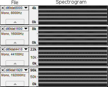
The files have different sample rates, and their spectrograms aren't exactly identical, but they all look basically the same: four strong and evenly-spaced peaks that stay constant over time. Actually, there's a fifth peak hiding at 0, and Audacity is hiding a mirrored half of the frequency spectrum. So really there are ten peaks. It is not a coincidence that the number of implied peaks is equal to the period of our input signal.
Keep in mind that each spectrogram in the above diagram has a different frequency scale. Varying the sample rate is having an effect on the frequency peaks: when the sample rate is twice as high, the frequencies are twice as high. But proportionally speaking the spectrograms have peaks in the same places, and that's what we care about.
(If you actually generate and play those audio files, you'll find that they do in fact sound like a constant tone made up of several frequencies.)
Now let's switch from periodic audio signals to periodic states on a quantum computer.
Periodic states and their frequencies
If you have a computer that can store 5 classical bits, there are 32 possible states that your computer can be in.
There's 00000, 00001, 00010, 00011, 00100, and so forth up to 11111.
One state for each way you can assign a 0 or a 1 to each bit.
The thing that separates a quantum computer from a classical computer is that a quantum computer can rotate its state through particular weighted combinations of the classical states (called "superpositions"). You can write down possible states of a 5-qubit quantum computer by adding together various proportions of the 32 classical states achievable with 5 bits, as long as the squared magnitudes of the weights add up to 1. So a 5 qubit quantum computer could be in the state $|00000\rangle$, or in the state $\frac{1}{\sqrt{2}}|00000\rangle + \frac{1}{\sqrt{2}}|11111\rangle$, or in the state $\frac{3}{5}|00000\rangle - \frac{4}{5}|10101\rangle$, or in the state $\frac{1}{\sqrt{3}}|00001\rangle - \frac{1}{\sqrt{3}}|00100\rangle + \frac{1}{\sqrt{5}}|10000\rangle$, or all kinds of other fun combinations.
In this post when I say "periodic state", I mean a superposition where the weights of the classical states go like 'zero, zero, zero, zero, NOT ZERO, zero, zero, zero, zero, NOT ZERO' and so forth. In other words, the classical states that have non-zero weight should be evenly spaced (and they should all have the same non-zero weight).
For example, the state $\frac{1}{\sqrt{7}} |00000\rangle + \frac{1}{\sqrt{7}} |00101\rangle + \frac{1}{\sqrt{7}} |01010\rangle + \frac{1}{\sqrt{7}} |01111\rangle + \frac{1}{\sqrt{7}} |10100\rangle + \frac{1}{\sqrt{7}}|11001\rangle + \frac{1}{\sqrt{7}}|11110\rangle$ is a periodic state. It gives $\frac{1}{\sqrt{7}}$ weight to the state 00000, to the state 00101, and so forth up to 11110. All the other states aren't given any weight. In decimal, the states with non-zero weight are 0, 5, 10, 15, 20, 25, and 30. This is a periodic state with a period of 5. A more compact way to write this state is with summation notation, like this: $\frac{1}{\sqrt{7}} \sum_{k=0}^{6}|5k\rangle$. The state $\frac{1}{\sqrt{7}} \sum_{k=0}^{6}|5k+1\rangle$ is another, different, periodic state with period 5.
At this point a certain subset readers are probably thinking something along the lines "Superposition? Bah! I bet the quantum computer is just secretly in one of those states with non-zero-weight, but we don't know which! How is this any different from a probability distribution?".
The answer to the "how know superpositions real?" question is: because we can operate on the states, and the outcomes of those operations differ depending on whether or not you started in a superposition of states or a single state (or in a probability distribution of states).
The specific quantum operation we care about in this post is the quantum Fourier transform (the QFT). What the QFT does is... it's like it takes the weights of the states, pretends they're the samples making up an audio file, figures out what the frequencies in that audio are, then uses the strength of each frequency as the new weights defining the state of the computer. (A good predictor for whether you even slightly understood that last sentence is whether or not your mind just got blown hard.) The point is: after applying the QFT, sampling the quantum computer's state can tell us what the dominant frequencies of the input state were (if any).
If you start with a classical state and apply the QFT operation, the resulting frequency spectrum looks completely flat (all the action is in the phases, not the magnitudes). By contrast, the frequency spectrum of a periodic signal is definitely not flat. Like the spectrograms from earlier, the frequency spectrums of periodic signals have sharp peaks. Furthermore, the number of frequency peaks isn't a property of some individual state. The number of peaks is equal to the spacing between states.
(If the quantum computer was really in just one of the classical states, how could a property about the spacing between the possible states be getting into the output? The frequency spectrums tell a very clear story about what's really going on.)
As a concrete example, I used my drag-and-drop quantum circuit simulator Quirk to prepare a periodic quantum state (more on that in a bit). Then I used a Quantum fourier transform operation to switch the state into its own frequency space. This is the result:
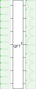
The green rectangle on the left is a "chance display". It's showing, for each classical state from 0000000 to 1111111, the probability that measuring the superposition at that point would return that state. You can tell the input state is periodic because the spikes in the chance display (corresponding to states with non-zero weights) are evenly spaced and all the same size.
The white box in the middle that says $\text{QFT}^\dagger$ is the (inverse) quantum Fourier transform operation. It switches the input state into its own frequency domain. I'm not going to get into exactly how the QFT is implemented under the hood. For the purposes of this post, all that matters is that it can be done. If you want more information, see the Wikipedia article.
The green rectangle on the right is a chance display showing the probabilities of getting various outcomes when measuring the output state. It has ten evenly-spaced peaks. Why ten? Because the number of frequency peaks is behaving just like it did with the periodic blip songs. The input state's period is ten, so the frequency space output has ten peaks.
Just to check that this is actually working, let's reduce the input state's period from ten to five. We should get half as many peaks:
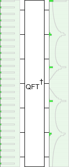
Yup, the output has a number of peaks equal to the period of the input.
Before we continue I want to address why we're bothering with frequency space at all. If we're after the period of the signal, why not just get it by looking directly at the input signal?
Keep in mind that the green displays in the diagrams are not available in real life. We don't get to see the distribution, we only get to sample from it. Sampling can efficiently tell us where various peak are (if they're tall enough), but not how many peaks there are.
Still, why don't we just sample the initial signal several times and watch for patterns? Why can't we figure out the period by sampling the input signal and noticing "Gee, there sure are a lot of multiples of 5 in here."?
The problem with noticing that a certain multiple keeps happening again and again is that, as you will see later, in the problem we care about, the signal we're sampling from is going to have a random offset. If we sample the number 213, that could be $50 \cdot 4$ with an offset of $13$ or $10 \cdot 21$ with an offset of $3$ or any other combination of offset and multiple. Every time we sample, there will be a different unknown offset. This prevents us from figuring out the underlying pattern. Sampling from input states with random offsets will look exactly like random noise.
The random offsets are what make working in frequency space useful, because frequency peaks aren't affected by offsets. When you shift a signal, you may apply a phase a factor to each frequency, but the magnitudes of those frequencies all stay the same.
To demonstrate this, I made yet another circuit in Quirk. This time I'm using an operation that adds larger and larger offsets into the input register before the QFT happens, with Quirk simulating what happens for each offset. Notice that, throughout the resulting animation, the input state is cycling yet the output peaks are staying perfectly still:
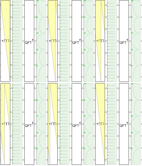
The phases of the output (not shown) are changing, but the magnitudes are staying the same. And, when ending a quantum computation, the magnitudes are what matter. The magnitudes determine the probability of measuring each state. (The phases matter if you're going to do more follow-up operations... but we aren't.)
Another thing you should notice in the above diagram is that the frequency peaks are resilient to little imperfections. Because the number of states ($2^7 = 128$) is not a multiple of the period ($5$), there's a little kink where the spacing between blips is 3 instead of 5. Despite that kink, the peaks are extremely close to 0/5'ths, 1/5'ths, 2/5'ths, 3/5'ths, and 4/5'ths of the way down the output space.
Preparing a periodic quantum state
I've explained that, if we had a periodic quantum state with unknown period, we could sample from the peaks in its frequency space in order to learn something about the period. But how do we prepare that periodic state in the first place?
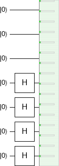
First, an easy case. If the period we want is a power of 2, let's say $2^3$, then preparing a periodic state is simple. Start with an $n$-qubit quantum register initialized to 0, do nothing to the first 3 qubits, and hit the rest of the qubits with a Hadamard gate. Each qubit you hit with the Hadamard gate will transition from the $|0\rangle$ state to the $\frac{1}{\sqrt{2}} |0\rangle + \frac{1}{\sqrt{2}} |1\rangle$ state, putting the overall qureg into the state $\frac{1}{\sqrt{2^{n-3}}} \sum_{k=0}^{2^{n-3}} |8k\rangle$. That's a periodic state with period $2^3$.
We can simulate this preparation in Quirk:
An alternative way to create a quantum state that has period 8 is to hit every qubit with a Hadamard gate, add the register we want to prepare into a register of size 3, then measure the other register and try again if the result isn't 0. Here's how that looks:
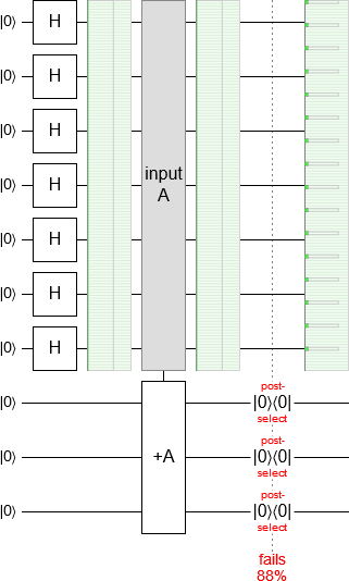
Beware that this is a case where the middle chance display is misleading. It looks like the addition didn't change to the state of the register we're preparing. Actually, its state was affected in a very important way.
One way to make the change caused by the addition more apparent is to use Quirk's density matrix display:
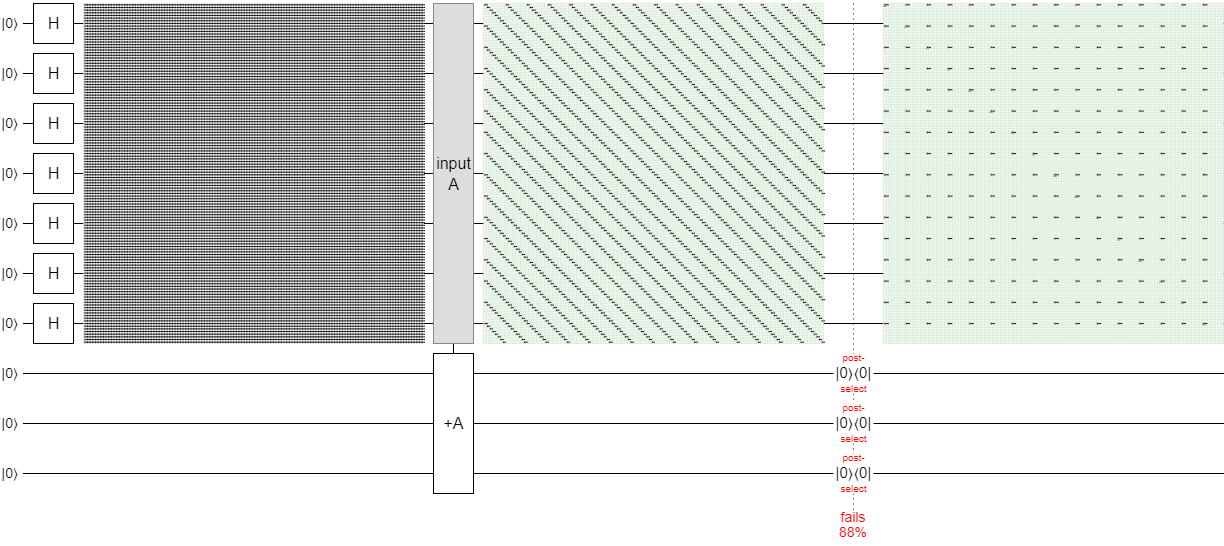
I don't expect readers to know how to read density matrices. The important thing to notice is that the addition turned the fine-grained grid pattern in the left display into a bunch of diagonal lines in the middle display. The diagonal lines are actually made up of a bunch of offset copies of more spaced out grids, like the one shown in the display on the right. Each of those offset copies represents a part of the superposition that can no longer interact with the other parts.
Let's call the top seven qubits the "input register" and the bottom three qubits the "ancilla register". When we add the input register into the ancilla register, we are basically copying the input register's value into the ancilla register, modulo 8 (because the ancilla register has 3 qubits and $2^3 = 8$). You can think of this as separating the input register's superposition into 8 parts, one for each remainder modulo 8. There's a part for the classical states whose remainder is 0, one part for values whose remainder is 1, one for remainder 2, and so forth up to the part for remainder 7.
If we were to measure the ancilla register, it would tell us something about the input register. Specifically, it would tell us which of the eight parts of the superposition survived. But, regardless of that measurement result, the surviving state is always a periodic quantum state with period 8. Only the offset of the state changes.
Note that, even if we haven't measured the ancilla register yet, it's reasonable for us to say "the input register contains a periodic quantum state with period 8". In fact that's reasonable to say even if we plan to just chuck the ancilla register away without bothering to measure it. It's the initialization of the ancilla register that split the input register into separate non-interacting pieces. The only practical difference between doing a "real" measurement and initializing that ancilla register is that a "real" measurement can't be undone but the ancilla register could be cleared by subtracting the input register out of it (...but we're not going to do that).
To convince you that the input register really does contain a periodic state, even if we don't condition on or measure the second register, let's make another circuit in Quirk. The frequency peaks don't move when you offset the input signal, so it really shouldn't matter that there's an unknown or even unmeasured offset. Prepare a uniform superposition in the input register, add into the ancilla register, Fourier-transform the input register, and...
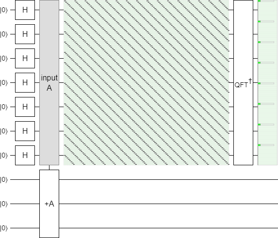
The peaks are there! We prepared a state with period 8 and, despite an unknown unmeasured offset, there are 8 peaks in its frequency spectrum. (The peaks are perfectly sharp spikes because both the period and the size of the QFT are powers of 2.)
I hope this really drives home how superpositions and probability distributions are different from each other. The input register effectively contains both types: it's in a probability distribution over the offsets of a superposition with period 8. And the various measurements and operations we can try clearly delineate between the probability part and the superposition part. In particular, the expected output changes if we measure the superposition part but not if we measure the probability part.
If we measure the ancilla register, that's like measuring the probability part. It tells us the offset of the periodic state. But, regardless of the outcome, the input register will still contain a superposition with period 8. The output frequency spectrum will still have 8 peaks in it.
Contrast this with what would happen if we measured the input register (before performing the QFT). The input register's state would collapse to some specific state $|k\rangle$. The frequency spectrum of a single state looks flat, so instead of seeing a number of peaks related to the period of the input state we'd see... flat.
In this animation, I use Quirk to sweep through the classical states and show their QFT outputs:
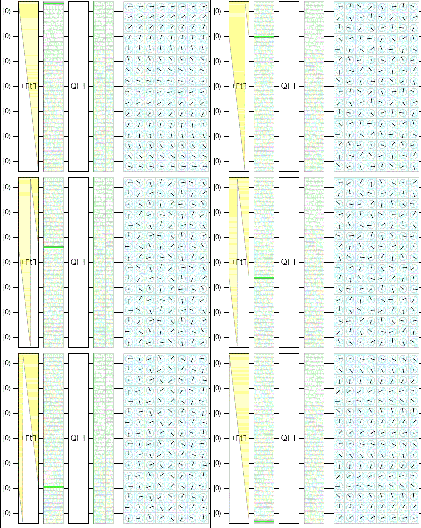
Notice that the output chance display is in fact staying flat. There's still plenty of fun stuff happening, but it's all going into rotating the phases of the amplitudes. (That's what's being shown in the cells of the pale blue rectangle.)
Measure the probability part, and nothing significant changes. Measure the superposition part, and you get a totally different style of output.
That's probably enough harping on the fact that superpositions just really don't behave like probability distributions. Let's move on to preparing states with other periods.
Preparing other periodic states
Instead of doing a three-bit addition, i.e. an addition modulo 8, we can do addition modulo some other number. This allows us to prepare a periodic quantum state with any period we want. The state we prepare will still have an unknown offset, but that's okay: the frequency peaks don't care.
For example, here is a circuit in Quirk that prepares a periodic quantum state with period 7, then applies a Fourier transform to show that there are 7 peaks in the output state:
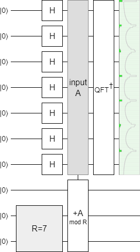
Yup, 7 peaks.
Now we have a general procedure for making periodic states with any period we want. We'll come back to this theme later, but first I want to explain how knowing the location of just one peak can tell you the period of the input. (As opposed to having to count the peaks, which would require quite a lot of sampling.)
Figuring out periods from frequency samples
Here's a bit of a puzzle for you. I'm going to show you a circuit that prepares a periodic state using a modular addition like in the last section, but I'm going to hide which modulus I'm using. Your job is to figure out the secret modulus.
Here's the circuit:
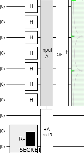
Do you know what $R$ has been set to?
It should be obvious: there's three peaks, so $R=3$.
But remember: when running an actual computation, we don't get to see the whole output state. We only get to see one measurement outcome at a time. If we ran the circuit enough times, we would get some rough idea of the number of peaks... but the amount of times we would have to run the circuit would scale with the number of peaks. If there were $P$ peaks, we'd need to do $O(\sqrt{P})$ runs before we had a reasonable idea of what $P$ was. This is a problem, because the input states we will be dealing with when factoring numbers will have huge periods. We need a faster way to do this, that works with fewer samples.
Suppose we were sampling from a frequency space of size $N=1024$, and that we didn't know the period of the input signal, but we got a frequency sample $s=340$. What do you think the secret period might be?
...
...
What if I told you the period was less than 6?
...
Okay, let me give you a hand by going over each case. If the period was 2, there should be two frequency peaks: one at 0, and one half-way across the space near 512. If the period was 3, there should be three frequency peaks: one at 0, one a third of the way across the space near 343, and another two thirds of the way across near 687. If the period was 4, there should be peaks near 0, 256, 512, and 768. If the period was 5, there'd be peaks near 0, 205, 410, 614, 819.
Did you see it? Only one of the periods has a frequency peak near our sampled frequency. If the period was 3 then there's a peak around 343. Our sampled value of $s=340$ is near 343. This means the input state's period was almost definitely equal to 3.
When the range of possible periods is huge, we can't simply go over all of the cases like we did here and see what's closest. We need a more clever strategy to find fractions near the point we sampled. This clever-er strategy comes in the form of the continued fractions algorithm for the best rational approximation.
I would explain exactly how that algorithm works, but python conveniently has it built into the fractions module.
We don't have to know how it works, we can just use it:
from fractions import Fraction
print(Fraction(340, 1024).limit_denominator(5))
# prints '1/3'
With limit_denominator in hand, it's easy to write a "sampled frequency to period" function:
from fractions import Fraction
def sampled_freq_to_period(sampled_freq, num_freqs, max_period):
    f = Fraction(sampled_freq, num_freqs)
    r = f.limit_denominator(max_period)
    return r.denominator
One pain point here is that our sample might be from the peak near 0. In that case we learn nothing, because every period has a peak near 0. That's fine, because getting 0 is really really unlikely for states that have a large period (which is the case we care about). And if we do get really unlucky... well, we can just try again. And if we keep getting values near 0 again and again and again forever, then I guess we win a Nobel prize because we found a repeatable experiment demonstrating that quantum mechanics is wrong.
The other thing to keep in mind, for quantum states that have potentially huge periods, is that the possible fractions start getting quite close together. If our maximum period is $p$, then the closest fractions are a distance of $1/p^2$ apart. So we need to make sure the frequency space we are sampling from is large enough to tell those fractions apart. Practically speaking, that means our input register must have at least $\lg p^{2} = 2 \lg p$ qubits.
When factoring a number $R$ with $N$ bits, the maximum period will be $2^N$ and we'll need $O(\lg 2^N) = O(N)$ qubits. Which is reasonable.
Preparing states with unknown periods
Modular addition isn't the only way to prepare periodic states. I mean, if it was, the ability to figure out the modulus by sampling the frequency space of the state would be an esoteric but ultimately pointless bit of trivia. Whoever put together the circuit obviously knew the modulus. They could have just told it to you instead of wasting time making you sample frequencies.
In order to do something interesting, we have to be able to make a periodic-state-producing circuit from start to finish and still not know what period its state will have.
It turns out that this is not very hard to do. We can use any periodic function $f$ to produce a periodic state, and there's no shortage of functions where figuring out the period is hard even if you know $f$. As long as $f(x)$ equals $f(x + p)$ regardless of $x$ for some $p$, and we can make a circuit that computes $f$, we can produce a periodic state that we can then sample in order to figure out $p$. The key point to internalize is that knowing $f$ doesn't mean you know $p$.
For example, suppose we use $f(x) = 2^x \pmod{23}$. What's the period of this function? In other words, if you start at 1 and begin multiplying by 2 again and again, how long will it be until you reach another number that's 1 more than a multiple of 23?
Let's try: 1 times 2 is 2, then 2 times 2 is 4, then 8, 16, 32→9, 18, 36→13, 26→3, 6, 12, 24→1; there it is! It took us... 11 doublings to get back to 1. So the period of $2^x \pmod{23}$ is 11.
Now let's try a different approach to the problem: preparing a periodic state and looking at its frequency spectrum. Open Quirk, create a uniform superposition for $x$, initialize the ancilla register to 1, multiply it by $2^x \pmod{23}$, and...
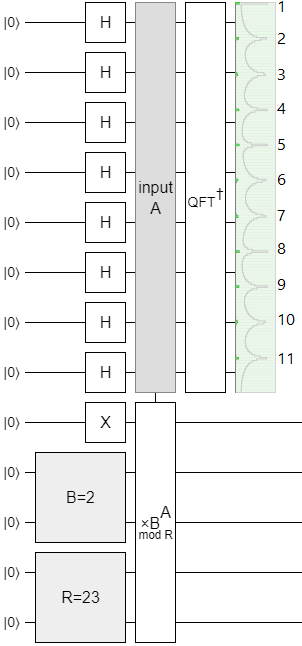
Eleven peaks! And we didn't have to double eleven times to figure that out.
Okay okay, let's try something a bit harder. This time we're going to be multiplying by 7 modulo 58, and I'm not going to show you the impossible-in-reality chance display. All you get is a sample:
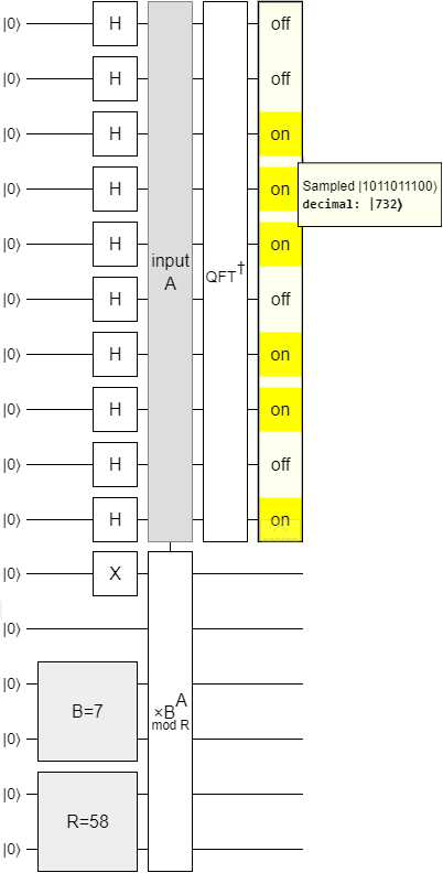
I promise I didn't cherry-pick the output shown in the diagram. I took a random sample. There were $2^{10} = 1024$ possible frequency samples, we got a sample of 732, and we know the period can't be more than our modulus of 58.
Given the sample from the diagram, can you figure out the period of $f(x) = 7^x \pmod{58}$ without multiplying by 7 until you get back to 1?
...
...
Hey, remember that sampled_freq_to_period python function we defined earlier?
...
...
Let's try it:
guess = sampled_freq_to_period(sampled_freq=732,
                               num_freqs=1024,
                               max_period=58)
print(guess)
# prints '7'
Pass our parameters into the function, and out pops 7. Feel free to check that $7^7 \pmod{58} = 1$.
At this point you should be convinced that, assuming we can actually implement this $\times B^A \pmod{R}$ operation from the diagrams, we can recover its period by sampling from a frequency spectrum and using our handy-dandy python function. (Explaining exactly how to efficiently implement a modular exponentiation operation on a quantum computer is way more detail than I want to go into. If you're really interested, I wrote a whole paper about it.)
The only real missing piece now is... why the heck are we computing this period?! What do we even do with it??
Answer: We're going to use it to find extra square roots.
Follow-up question: What? How does that help us factor numbers? What even is that?! Why are there so many steps! Why is this so hard!? Auuuurrrrgh!!
Answer: Uh... okay. Look, just hold on, we're getting there. I promise.
Turning an extra square root into a factor
An "extra square root" is a number $u$ that squares to give 1 and yet isn't +1 or -1. In the number systems you're probably used to, this never happens. But, in modular arithmetic, it does. For example, when working modulo 100, the number 49 is an extra square root. 49 isn't 1, and it isn't 99 (which is -1 mod 100), but $49^2 = 2401 \equiv 1 \pmod{100}$.
The thing about knowing $u^2 = 1$ is that we can rewrite this equation into $u^2 - 1 = 0$. That equation factors. It's equivalent to saying that $(u-1)(u+1) = 0$.
Now, if $u$ was 1, the fact that $(u-1)(u+1) = (1-1)(1+1) = 0 \cdot 2$ was zero would not be very surprising. Similarly, if $u$ was -1, then $(u-1)(u+1) = (-1-1)(-1+1) = -2 \cdot 0$ vanishing is not very surprising. That's why we need an extra square root: to make the equation $(u+1)(u-1) = 0$ actually interesting.
If we're working modulo $R$, then knowing $(u-1)(u+1) = 0$ tells us that in the usual integer arithmetic $(u-1)(u+1)$ is a multiple of $R$. In other words, we know two non-zero values, $a = u-1$ and $b = u+1$, such that $a \cdot b = k \cdot R$ for some integer $k$.
Suppose we factorized $a$, $b$, $k$, and $R$ into their prime factors. Then our equation becomes:
$$(a_1 \cdot a_2 \cdot ... \cdot a_{n_a}) \cdot (b_1 \cdot ... \cdot b_{n_b}) = (k_1 \cdot ... \cdot k_{n_k}) \cdot (R_1 \cdot ... \cdot R_{n_R})$$
Every prime factor that appears on the right hand side of that equation must have partner on the left hand side. But here's the thing: the partners to the prime factors in $R$ have to be spread over both $a$ and $b$. If all of $R$'s prime factor partners were in $a$, then $a$ would be a multiple of $R$. Which would mean $u-1$ was zero the whole time (modulo $R$). Which would violate our assertion that $u$ isn't congruent to 1. The same logic applies to $b$.
So we know $a = u-1$ has some factors in common with $R$. That's great, but $a$ might also have factors in common with $k$. We need to filter those out. Fortunately, this is easy: we just compute the greatest common divisor of $R$ and $a$.
What we're left with is a number $r = \text{gcd}(u-1, R)$ that has prime factors in common with $R$, but can't have all the prime factors in $R$. Therefore $r$ is a factor of $R$.
For example, recalling the $49^2 = 1 \pmod{100}$ example from the start of this section, we find that $\text{gcd}(49-1, 100) = 4$. And 100 is in fact divisible by 4.
Turning a period into an extra square root
So, we know how to take an extra square root $u$ modulo $R$, and turn that into a factor of $R$. We also know how to use a quantum computer to tell us the period of the function $f(x) = B^x \pmod{R}$ for any base $B$ and modulus $R$. How do we put these two pieces together?
Well... the period $p$ is the smallest solution to the equation $B^p = 1 \pmod{R}$. The key idea is that, if we raise $B$ to half of the period, then the result will be a square root of $1$. After all, $B^{p/2} \cdot B^{p/2} = B^p$ and we already know that $B^p = 1 \pmod{R}$.
Sometimes the square root we get will be -1, instead of an extra square root. Sometimes the period will be odd, so we won't be able to divide it in half. But, not infrequently, the period will be even and $B^{p/2}$ won't be congruent to -1. Then we win.
The good case isn't rare, by the way. As far as I know, it's akin to winning two coin flips. We might have to try a few random $B$'s before landing on one that works, but when we do... bingo.
Putting it all together
We've now discussed all the key parts of Shor's algorithm:
- Using a quantum computer and frequency space sampling to perform period finding.
- Using period finding to find extra square roots.
- Using extra square roots to get factors.
With all of this information internalized, we can finally write some pseudo-code to simulate Shor's algorithm:
from math import log2
from fractions import Fraction, gcd

def factor_attempt(n):
    base = random.randint(2, n-2)
    period = sample_period(base, n)

    # Try to extract an extra square root.
    half_period = period // 2
    u = pow(base, half_period, modulus)
    if u == 1 or u == n-1 or u**2 % n != 1:
        return None  # Failed attempt.

    # Use extra square root to pull out a factor.
    return gcd(u + 1, n)


def sample_period(base, modulus):
    modulus_bit_count = int(ceil(log2(modulus)))
    precision = modulus_bit_count * 2

    # Prepare a uniform superposition of possible exponents.
    exponent_qureg = Qureg(size=precision, initial_value=0)
    for q in exponent_qureg:
        apply Hadamard to q

    # Create distinguishing information that separates the exponents
    # into equivalence classes modulo the unknown period.
    ancilla_qureg = Qureg(size=modulus_bit_count, initial_value=1)
    ancilla_qureg *= pow(base, exponent_qureg, modulus)

    # Convert to frequency space.
    apply QFTinv to exponent_qureg

    # Sample from the frequency spectrum.
    s = measure exponent_qureg

    # Figure out the fraction closest to the proportional sample.
    frac = Fraction(numerator=s, denominator=1 << precision)
    nearby_bounded_frac = frac.limit_denominator(modulus - 1)

    # The denominator should be the period.
    return nearby_bounded_frac.denominator
The above code is really just a more detailed version of the flowchart from earlier:
Still, even with the extra details, I'm simplifying quite a lot. A real algorithm would break down the exponentiation into basic quantum gates. It would also check several fractions and periods near to the sampled value, in case the sampled result was close instead of exact. It would deal with special cases like "Oops, I'm an extremely lucky person and the base I chose at random isn't co-prime to the modulus.". It would check for various classically-easy cases like small factors and square numbers. And so on and so on.
End to end example
We have all the pieces we need, let's apply them.
I went to a list of all the primes up to a million, picked two at random, and multiplied them together. The result was:
$R = 75945260669$
We're going to factor this number using Shor's algorithm. Unfortunately we can't use a quantum computer to do it. But the numbers are small enough that we can brute-force the period finding classically:
def brute_force_find_period(B, R):
    n = 1
    t = B
    while t != 1:
        t *= B
        t %= R
        n += 1
    return n
Just... be prepared to wait a few minutes for that method to run, okay?
We start Shor's algorithm by picking a random base $B$.
I ran B = random.randint(0, R) in python and got:
$B = 58469529322$
Now we want to know the period of $f(x) = B^x \pmod{R}$, so we run brute_force_find_period(B, R).
This is the slow step classically, and it takes a couple minutes for the naive brute force search we're using to finish.
Using the classical method means we don't get to practice the period-from-closest-fraction's-denominator thing.
You'll have to do that on your own.
Anyways, eventually we get our answer:
$P = 327347592$
The period is even, which is good because we need that.
Otherwise we'd have needed to retry.
However, we'll also need to retry if $B^{P/2}$ is congruent to $R-1$.
I ran u = pow(B, p // 2, R) and... we got lucky!
The result wasn't $R-1$; we found an extra square root:
$u = 23766570031$
(You can check that u**2 % R spits out 1, as it should.)
Now we know that $(u-1) \cdot (u+1) = 23766570030 \cdot 23766570032 = k \cdot R$ for some unknown integer $k$.
All we need to do is use gcd to filter the unknown $k$'s prime factors out of $u-1$ or $u+1$, and we're home free.
We run r1 = fractions.gcd(u-1, R) and get our first factor:
$r_1 = 450893$
We can get the second factor by dividing $R$ by $r_1$ or by running fractions.gcd(u+1, R).
Either way we find that:
$r_2 = 168433$
We then check our answer with print(r1 * r2 == R):
True
We did it! $r_1$ and $r_2$ are in fact the two primes I picked. $75945260669$ factors into $168433 \cdot 450893$.
Conclusion
Shor's algorithm is difficult to understand because it mixes together ideas from quantum physics, signal processing, number theory, and computer science. I didn't cover all of the details, but I hope I got across the basic ideas needed to understand the pieces and how they fit into a coherent algorithm for factoring numbers.
Acknowledgements
I'd like to thank Bernardo Meurer for proof-reading this post and pointing out several places where the explanations were seriously lacking.

