

This post will cover two things. First, we'll go over a particularly nice way of performing classical roulette selection. Second, we'll enter quantum land and I'll explain how the improved roulette selection method allowed me and some collaborators to make a key element of quantum chemistry simulations a lot faster.
Update (June 2018): I presented on this topic at the joint session of QPL 2018 and MFPS 2018. The talk wasn't recorded, but you can view the slides (or as a pdf).
Roulette Selection
If you've ever written a genetic algorithm, you've run into roulette selection. Basically, there comes a point where you want to randomly choose which genomes will advance to the next generation, and you want to pick genomes that scored well more often. In the simplest case, if genome A has twice as much fitness score as genome B then A should be sampled twice as often as B. When you write code that does that kind of sampling, you're writing a roulette selection algorithm.
Roulette selection is often called "fitness proportionate selection" or "proportional selection" because the probability of selecting a thing is proportional to its probability. If you apply a bit of google-fu to those terms, you'll find a nice web page by John Bjorn Nelson that goes over different roulette selection algorithms. The page covers three methods:
Linear walk. Add up the fitness scores of every item, generate a random number between 0 and the total score, then iterate through the list while subtracting each item's score from the generated number. Just before you cross into negative territory, return the item you're on.
Bisecting search. Precompute a balanced search tree over the cumulative fitness scores. Use the tree to quickly find at which item the transition into negative territory would occur during a linear walk. Generate a random number between 0 and the total score , use the tree to quickly find the transition, and return the appropriate item.
Stochastic acceptance. Pick an item uniformly at random. Return it with probability $f_{\text{item}} / f_{\text{max}}$, otherwise try again.
All three of these methods need $O(n)$ precomputation, where $n$ is the number of items. The linear walk methods needs to compute the total fitness, which takes $O(n)$ time. The bisecting search method needs to prepare the search tree, which also takes $O(n)$ time. And the stochastic acceptance method needs to compute the maximum fitness; $O(n)$ time yet again.
Where these methods differ is in how much time they take to generate a sample. The linear walk method needs $O(n)$ expected time to produce a sample (because you tend to travel over half of the items looking for the one that was actually chosen). The bisecting search method uses a search tree to improve the sample time to $O(\lg n)$. Stochastic acceptance has a bit of a strange runtime: $O(nf_{\text{max}} / f_{\text{total}})$. Basically, it is very fast when your distribution of fitnesses is nearly uniform but if you have any outliers it quickly degrades to $O(n)$ time.
There are optimizations you can do when producing many samples to make these numbers better, but for the purposes of this post we only care about producing one sample. For comparison purposes, I have included a table below summarizing the cost of each method. The last row, "subsampling", is the method I will explain in the next section.
| Method | Precompute Time | Space Usage | Expected Sampling Time |
|---|---|---|---|
| Linear Walk | $O(n)$ | $O(1)$ | $O(n)$ |
| Bisecting Search | $O(n)$ | $O(n)$ | $O(\lg n)$ |
| Stochastic Acceptance | $O(n)$ | $O(1)$ | $O(n f_{\text{max}} / f_{\text{total}})$ |
| Subsampling | $O(n)$ | $O(n)$ | $O(1)$ |
(Note that subsampling dominates bisecting search. It even has lower constant factors hiding behind the asymptotic notation!)
Subsampling
The key idea behind subsampling is that it is possible to split our big sampling problem into a collection of equally-likely subproblems, where each subproblem only involves choosing between two items.
Basically, we're going to take a histogram, like this one:
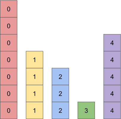
Then we're going to permit every bar to have two colors instead of one, which will allow us to rearrange the histogram so that every bar has exactly the same height:
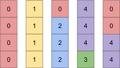
If you check closely, you'll see that the repacked histogram has exactly the same number of squares of each type as the original histogram. This suggests a very efficient way to sample the items in a fitness-proportionate way: pick a bar, then pick a color within the bar.
Let's do an example. We start by picking pick one of the bars uniformly at random. For example, suppose we pick the middle bar. Then we'll check which colors are in the bar we picked and how many of each color there are. The bar we picked has three blues and one red. Finally, we randomly pick between the two colors with a probability based on how many of each there are. Our chosen bar has three blues to one red, so we should return blue with 3:1 odds (i.e. three quarters of the time) and otherwise red.
Here is the subsampling procedure, slightly streamlined, implemented in python:
import random

def subsample(colors, alternate_colors, bottom_proportions):
    # Pick a bar uniformly at random.
    bar = random.randint(0, len(items))

    # Look up colors and relative weight of each color.
    bottom_color = colors[bar]
    top_color = alternate_colors[bar]
    bottom_color_proportion = bottom_proportions[bar]

    # Pick between the two colors with the appropriate probability.
    if random.random() < bottom_color_proportion:
        return bottom_color
    return top_color
This is a very straightforward "do this then do that then do that" process. There's no loops, no complicated conditions, just bang bang bang done. The tricky part is all hidden away in the repacking process, which is of course key to making this whole thing actually work.
Mathematically speaking, the goal of the repacking process is to find probabilities $\text{keep}_k$ and values $\text{alt}_k$ that satisfy the following contract for all values $k$:
$$\frac{1}{n} \left( \text{keep}_k + \sum_{i | \text{alt}_i = k} 1 - \text{keep}_i \right) = \frac{\text{fitness}_k}{\text{fitness}_\text{total}}$$
But I think this is a clear example of a problem that should be approached using visual intuition, instead of with algebra. So here's how you solve this problem, in diagram form.
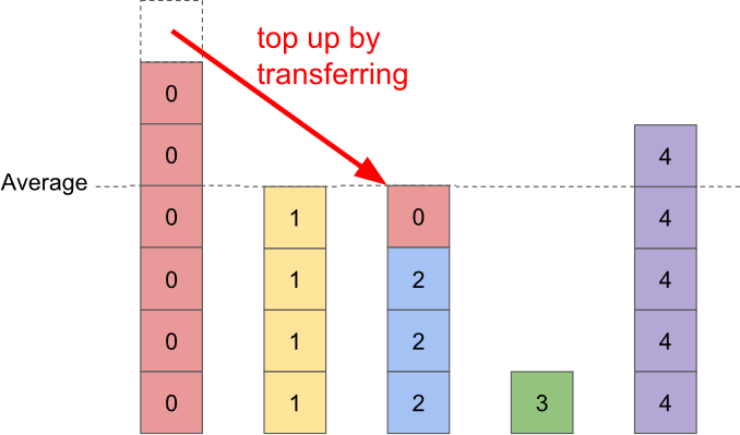
1) Create a histogram representing your problem. Add in an indicator showing the average height of the bars.
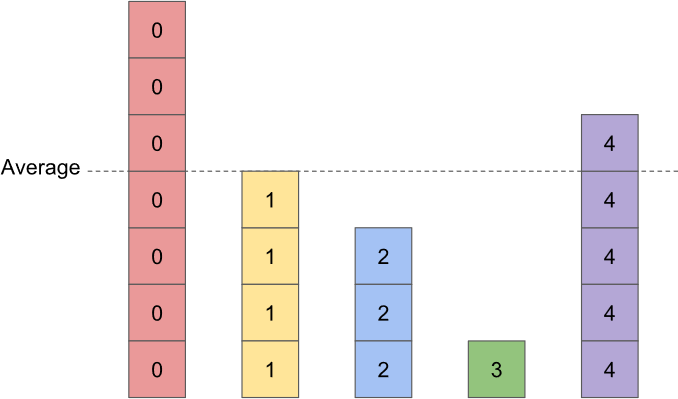
2) Pick a bar that's below the average value. If there isn't one, you're done. If there is, find a second bar that's above the average value. (There will always be one.) We're going to use the above-average bar as a donor for the below-average bar.
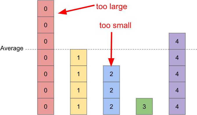
3) Transfer weight from the above-average bar to the below-average bar until it is exactly the right height. This permanently solves the (previously) below-average bar.
4) Goto step 2.
Note that it is possible for the topping-up process to cause the above-average bar to become a below-average bar. In fact, it will happen in the next iteration no matter which bars we pick:
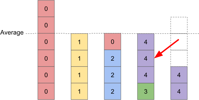
This is totally fine; it will be dealt with in later iterations. In the example case I've been diagramming, the very next iteration fixes the problem and completes the solution:
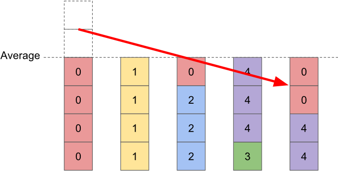
What's important here is that every time we do an iteration, i.e. every time we transfer probability, a below-average bar is topped up to exactly the average value and then stays there. This effectively leaves us with a smaller version of the original problem, which guarantees we won't end up stuck in a loop or in a dead-end. If we start with $n$ bars, then every bar will be exactly the same height after at most $n-1$ iterations.
Notice that the solution we found above is not unique. If you choose different too-high-too-low pairs while executing the algorithm, you'll end up with a different solution. In general, there will be many many possible solutions. Sometimes even more than $n!$, which is a lot!
The strategy you use for picking too-high-too-low pairs will determine the runtime of the repacking algorithm. If you naively rescan the remaining bars every time, the runtime will be $O(n^2)$. If you use a priority queue or a search tree to ensure you can always quickly find the smallest and largest bars, the runtime will be $O(n \lg n)$. And if you're just a tiny bit more clever, you can get the runtime down to $O(n)$.
I'll leave figuring out an $O(n)$ algorithm as a challenge for the reader, and move on to quantum computing.
Update (May 21): I figured there must be pre-existing work that covered subsampling, but I couldn't cite it because I didn't know what it was called! Fortunately for me, commenter 'notfancy' did. They pointed out that "subsampling" is more commonly called "the alias method" and that the linear time algorithm for generating the index used by the alias method is called Vose's algorithm (see the 1991 paper "A linear algorithm for generating random numbers with a given distribution").
Preparing Superpositions
In the paper "Encoding Electronic Spectra in Quantum Circuits with Linear T Complexity", there is a particular task that we need to perform millions of times: preparing a superposition with specified amplitudes. It doesn't really matter where those specified amplitudes come from (it's some big complicated equation). What matters is getting the job done fast.
Previously, the way people would approach this problem was in many ways equivalent to the bisecting search approach to roulette selection. You would start with the most-significant qubit, look at your precomputed table of amplitudes in order to determine the proportion of that-qubit-is-ON cases vs that-qubit-is-OFF, then rotate the qubit by exactly the right amount to get the correct proportion. Then you'd go to the next most significant qubit and repeat the process, but once conditioned on the most significant qubit being ON and once conditioned on it being OFF (since the proportion may depend on the value of the most significant qubit). You would continue to dig down through the qubits, conditioning on all the possible cases, until you had processed the least significant bit.
The problem with the approach described in the above paragraph is two-fold. First, rotating by weird angles is not cheap. An early error corrected quantum computer could easily spend several milliseconds on each of those rotations. Second, we're using a tree structure but not really getting any benefits from it. Classically, tree-based methods are great because you only have to go down one path. So you pay an amount proportional to the depth of the tree, which is typically $O(\lg n)$. Quantumly, you have to go down a superposition of paths. If you want a path to work, you have to apply all the operations needed by that path. Since we want every path to work, we need to apply the operations for every path and end up doing an amount of work proportional to the size of the tree.
Still, despite those problems, for a long time we weren't able to see a better way to get this done. And, actually, I still don't know a better way to do it. You see, sometimes, when you're given a problem, the correct approach is to realize it's the wrong problem.
In the paper, the superposition we want to prepare is used in a very specific way. It is used to control operations being applied to a system state register, and then uncomputed. That's it. There are no operations targeting the superposition, it is only used as a control register. We prepare the superposition, control some operations with it, then unprepare it using exactly the opposite procedure that was used to prepare it.
The key insight here is that under these conditions, it doesn't matter if we mess up the phases of the superposition. Phase error on a qubit commutes with operations where that qubit is only used as a control. Therefore phase error during preparation will commute across the intermediate operations, and cancel against exactly-opposite phase error during unpreparation. If we mess up the phases during prepare it won't hurt the controlled operations, and because unprepare is exactly the opposite of prepare it will fix the temporary phase error.
The reason this is a key insight is because it implies we can have registers that are entangled/correlated with the prepared superposition. Normally that kind of thing is fatal to a quantum algorithm. It's classical algorithms that can spread correlated data around willy-nilly, without ruining everything. This basically means that, because we are insensitive to phase error, we can use preparation strategies that would normally only make sense in a classical algorithm. In a certain sense, our superposition-preparing problem has turned into a much easier probability-distribution-preparing problem. The preparation process we use must still be reversible, but that's trivial to do: just keep track of any junk you produce.
Which brings us to subsampling.
Classically, we do subsampling by:
- Precomputing alternative items and keep probabilities for the desired probability distribution.
- Choosing an item uniformly at random.
- Looking up that item's keep probability and alternative item.
- Choose a threshold between 0 and 1 uniformly at random.
- If the threshold is less than the keep probability, return the item you chose. Otherwise return the alternate item.
And here is the quantum equivalent:
- Precompute alternative items and keep probabilities for the desired superposition (square the amplitudes to get probabilities).
- Prepare a uniform superposition over the possible item indices.
- Do a lookup (under superposition) of the keep probability and alternative item.
- Prepare a uniform superposition over values between 0 and 1 (using fixed-point arithmetic at some target precision).
- Compute (under superposition) whether the value from (3) is less than the value from (2).
- If so, swap the values of the register storing the chosen item (from 1) and the register storing the alternative item (from 2).
- The register from 1 is the result.
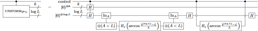
The processes are essentially identical, modulo "choose uniformly at random" turning into "prepare a uniform superposition". Here is a circuit diagram of the quantum process, from the paper:
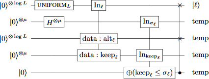
And for completeness here is a slightly magical circuit showing how you do the uniform superposition preparation steps cheaply:
Now let's compare the cost of this new method to the cost of the method that was more like bisecting search. This amounts to counting how many T gates they each use.
The bisecting search method has to do $n$ controlled rotations by specific angles. The number of T gates required to perform a rotation by a weird angle depends on how precise you're trying to be; if you have an absolute error tolerance of $\epsilon$ then the number of T gates needed to do the rotation well enough is $O(\lg 1/\epsilon)$. Taking into account the constant factors hidden by the asymptotic notation, and the values of $\epsilon$ that are realistic for a chemistry algorithm, this amounts to on the order of fifty T gates per rotation.
The dominant cost of the subsampling process is, somewhat surprisingly, looking up the keep probabilities and alternative items under superposition. If there are $n$ possible items, the T-count of the lookup is $4n$ (the method for doing the lookup this efficiently is explained in the paper). The cost of preparing the uniform superpositions is tiny in comparison; in fact it costs nothing at all if $n$ is a power of 2.
Using a subsampling-like method instead of a tree-like method reduces our dominant cost from ~50n to ~4n. That's over an order of magnitude better! This improvement, along with several others, is why the algorithm in our paper is a million times more T-count efficient than previous work. Despite being way (way) more conservative in our estimates, we reduced the execution times from months to hours while also reducing space usage by a factor of 10.
Closing Remarks
Subsampling repacks histograms in a way that allows roulette selection samples to be performed in constant time.
Subsampling strictly dominates roulette selection methods based on using a search tree.
By using a quantum variant of subsampling, you can do quantum chemistry simulations a whole lot faster.
Preparing superpositions is a lot easier when you're insensitive to phasing.
