

In a previous post, I explained how using quantum phase estimation on an operation can provide a mechanism for applying fractional powers of that operation. The basic idea being that the register containing the phase estimation acts as an index into the eigenspaces of the operation, allowing you phase those spaces by appropriate amounts.
A few days ago I was thinking in the shower and an idea occurred to me: what would happen if I used that same trick, but in the opposite direction? Instead of using phase estimation to apply tiny powers of an operation, let's try to use it to apply big powers of operations. Apply the operation $x$ times to compute the phase estimation, then use the phase estimation to apply the operation $t \gg x$ times.
Will it work? Probably not. But there's only one way to find out.
Experiment
When you have an idea, it pays to just try it. Do a quick experiment to see how things actually behave, before bothering with too much mathematical analysis. So, with that principle in mind, I opened up Quirk.
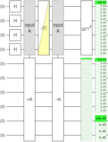
To keep things simple, I decided to try my idea on the increment operation. I arbitrarily decided to use 4 qubits for the phase estimation register, and 6 for the target register. I prepared the phase estimation register into a uniform superposition, used it to control how many increments happen (up to 16), and applied the inverse Fourier transform to get the phase estimates:
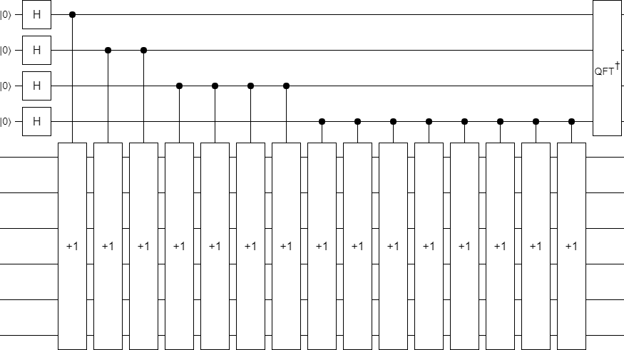
In the general case, the amount of repetition of the target operation shown in the above diagram is likely necessary. But it certainly isn't necessary for incrementing.
When you apply an increment twice to the same register, that's equivalent to doing a single shifted incremented. Iteratively merging doubled-up increments makes the circuit a lot more compact:
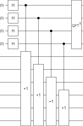
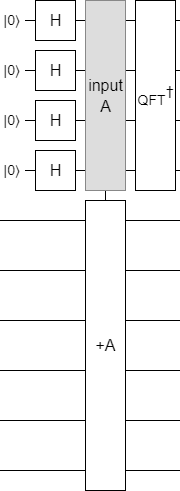
Actually, the above circuit is still kinda dumb. We're going over each bit of the input, and if it's set then we're adding 1 at that bit position into the target. Another name for this operation is "addition". Let's just do that:
With the phase estimation part of the circuit done, I applied a time-varying phase gradient to the phase register, uncomputed the phase estimation by mirroring the circuit, and added a display to see how well things were working.
The result was... underwhelming. We want to see the state smoothly sweep across the output display, but instead this is what happens:
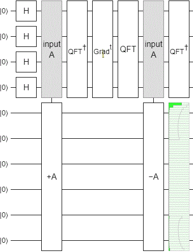
The "pumping" up and down is typical of what happens when you change incrementing into a continuous operation via its eigenvalues. But the gradual decay and leaking from the low part into the high part is not good at all. We want a strong peak smoothly pumping its way across the space, not a peak that dies out before even getting to the halfway mark.
To get a bit more insight into what was going on, I did three things to the circuit.
First, I noticed that the QFT+Gradient+QFT chunk at the center of the circuit could be simplified into a subtraction. That's because Fourier transforms translate between phase-gradients and additions, and for this particular problem we only care about integer powers. Making this change removes that visually distracting pumping motion from the output display.
Second, I looked more closely at how the individual qubits were being changed by the operation (not shown in the diagram above). There was a noticeable difference between how the bottom four bits and the top two bits were bouncing around, so I added separate displays for each of those ranges.
Third, I added a display for the phase estimation register. At first this wasn't showing anything interesting, but that's only because all the bad stuff was affecting only the phases of the state. I prefixed the display with a Fourier transform to fix that.
After those changes, the circuit cycled like this:
Basically what's happening here is that the operation works okay within the range we actually explored while doing the phase estimation, but it is failing at emulating the higher order changes. The low bits are behaving perfectly, but the high bits are merely rotating and leaking into the phase estimation register.
I should point out that, with the circuit simplified in this way, it's really obvious that this idea couldn't possibly work. The phase estimation register is smaller than the target register; we're trying to cycle through $2^6$ states by cycling through $2^4$ states, which makes no sense. Honestly it's impressive that the high bits are doing anything even slightly sensible.
For more insight into why this idea isn't working, we should do some error analysis.
Theory
We have a unitary operation $U$ with an eigendecomposition $U = \sum_{k} |\lambda_k\rangle\langle\lambda_k| \cdot e^{i \theta_k}$. We want to apply $U$ to a state $|v\rangle$. The state $|v\rangle$ can be decomposed into $U$'s eigenbasis as $|v\rangle = \sum_{k} |\lambda_k\rangle \cdot v_k$.
We want to apply $U$ to $|v\rangle$ a total of $t$ times. So, algebraically, our desired output state is:
$$ \begin{align} |\psi_{\text{desired}}\rangle &= U^t \cdot |v\rangle \\&= \left( \sum_{k} |\lambda_k\rangle\langle\lambda_k| \cdot e^{i \theta_k} \right)^t \cdot \left( \sum_{k} |\lambda_k\rangle \cdot v_k \right) \\&= \left( \sum_{k} |\lambda_k\rangle\langle\lambda_k| \cdot e^{i t \theta_k} \right) \cdot \left( \sum_{k} |\lambda_k\rangle \cdot v_k \right) \\&= \sum_{k} |\lambda_k\rangle \cdot e^{i t \theta_k} \cdot v_k \end{align} $$
Instead of applying $U$ directly, we're using the phase estimation procedure to estimate the various eigenvalues $|v\rangle$ is being decomposed into, and then phasing by those amounts. This introduces two kinds of errors into the phases of the eigenvalues we're using: spreading and rounding.
By "rounding" I just mean that the estimated eigenvalue angles are always a multiple of $2^{-p}$, where $p$ is the bit precision of our phase estimation. We're forcing a continuous spectrum into a discrete bunch of buckets.
By "spreading", I mean that the estimated eigenvalues will have a non-zero standard deviation. Most of the estimated value will concentrate near the true value, but there will be (negligible) components arbitrarily far away. For example, consider the following circuit:
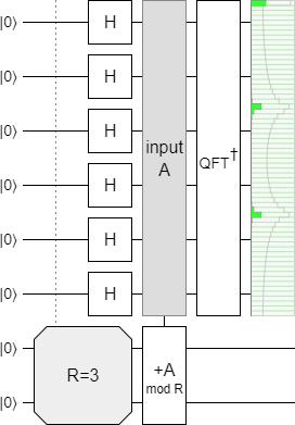
The $+A \pmod{3}$ operation has eigenvalue angles of $\theta_0 = 0$, $\theta_1 = \frac{\tau}{3}$, and $\theta_2 = \frac{2 \tau}{3}$: The value $2^n/3$ is not an integer, so the eigenvalue angle $\frac{\tau}{3}$ doesn't correspond to a single bucket in the phase estimation register, and so ends up both rounded and smeared. The amplitudes of the estimate are concentrated around the true eigenvalues, but the distribution that the phase estimation register's state corresponds to has a non-zero standard deviation.
To keep the math simple, I am going to completely ignore spreading and focus entirely on rounding error. I will assume that the phase estimation is magically off by exactly $\epsilon_k$ for the $k$'th eigenvalue, instead of a superposition of various offsets. This will give us a reasonable lower bound on how bad the estimated operation performes.
Given the no-spreading simplication, the state we'd actually be computing would be:
$$ \begin{align} |\psi_{\text{actual}}\rangle &=\text{PhaseEstimate}(U)^t \cdot |v\rangle \\&\approx \left( \sum_{k} |\lambda_k\rangle\langle\lambda_k| \cdot e^{i (\theta_k + \epsilon_k)} \right)^t \cdot |v\rangle \\&= \sum_{k} |\lambda_k\rangle \cdot e^{i t (\theta_k + \epsilon_k)} \cdot v_k \\&= \sum_{k} |\lambda_k\rangle \cdot e^{i t \theta_k} \cdot v_k \cdot e^{i t \epsilon_k} \end{align} $$
In order to determine how well the actual state approximates the desired state, we compute the trace distance between them. This will tell us how easy it is for an adversary to distinguish between the two states.
To start, we unpack the definition of the trace distance and simplify:
$$ \begin{align} \text{TraceDistance}(|\psi_{\text{desired}}\rangle, |\psi_{\text{actual}}\rangle) &= \frac{1}{2} \text{Tr} \; \text{abs}( |\psi_{\text{desired}}\rangle \langle\psi_{\text{desired}}| - |\psi_{\text{actual}}\rangle \langle\psi_{\text{actual}}| ) \\&\approx \frac{1}{2} \text{Tr} \; \text{abs}\left( \sum_{k} |\lambda_k\rangle\langle \lambda_k | \cdot e^{i t \theta_k} \cdot v_k - \sum_{k} |\lambda_k\rangle \cdot e^{i t \theta_k} \cdot v_k \cdot e^{i t \epsilon_k} \right) \\&= \frac{1}{2} \text{Tr} \; \text{abs}\left( \sum_{k} |\lambda_k\rangle\langle \lambda_k | \cdot (e^{i t \theta_k} \cdot v_k - e^{i t \theta_k} \cdot v_k \cdot e^{i t \epsilon_k}) \right) \\&= \frac{1}{2} \sum_{k} \text{abs}(e^{i t \theta_k} \cdot v_k - e^{i t \theta_k} \cdot v_k \cdot e^{i t \epsilon_k}) \\&= \frac{1}{2} \sum_{k} \text{abs}(e^{i t \theta_k} \cdot v_k \cdot (1 - e^{i t \epsilon_k})) \\&= \frac{1}{2} \sum_{k} |v_k| \cdot |1 - e^{i t \epsilon_k}| \end{align} $$
Then we assume that $\epsilon_k$ is small enough that a few approximations apply:
$$ \begin{align} \text{TraceDistance}(|\psi_{\text{desired}}\rangle, |\psi_{\text{actual}}\rangle) &\approx \frac{1}{2} \sum_{k} |v_k| \cdot |1 - e^{i t \epsilon_k}| \\&\approx \frac{1}{2} \sum_{k} |v_k| \cdot |\sin t \epsilon_k| \\&\approx \frac{1}{2} \sum_{k} |v_k| \cdot |t \epsilon_k| \\&= \frac{1}{2} t \sum_{k} |\epsilon_k| |v_k| \end{align} $$
Next, to bound the approximated distance, we assume that the magnitude of each error $\epsilon_k$ is below some fixed maximum error $\epsilon$:
$$ \begin{align} \text{TraceDistance}(|\psi_{\text{desired}}\rangle, |\psi_{\text{actual}}\rangle) &\approx \frac{1}{2} t \sum_{k} |\epsilon_k| |v_k| \\&\leq \frac{1}{2} t \sum_{k} \epsilon |v_k| \\&= \frac{1}{2} t \epsilon \sum_{k} |v_k| \end{align} $$
Finally, to get a bound that doesn't depend on $|v\rangle$, we look at the worst-case scenario for that sum. The worst case scenario is when $|v\rangle$ is exactly diagonal to the eigenbasis, meaning for $n$ qubits there will be $N = 2^n$ values of $|v_k|$, each with amplitude equal to $\frac{1}{\sqrt N}$. That gives us a worst case bound of:
$$\text{TraceDistance}(|\psi_{\text{desired}}\rangle, |\psi_{\text{actual}}\rangle) \lessapprox \frac{1}{2} t \epsilon 2^{n/2}$$
The above equations tells us that, if we want to use this phase estimation technique to apply an operation $t$ times with an overall error of at most $\delta$, our phase estimation error $\epsilon$ will need to be bounded below $\frac{2 \delta}{t 2^{n/2}}$. If we do a $p$-bit phase estimation, we bound $\epsilon$ below $2^{-p}$. That means $p$ must be at least $-\lg \frac{2 \delta}{t 2^{n/2}}$ or, more simply, $p \geq n/2 - 1 + \lg t + \lg \frac{1}{\delta}$.
See the problem? We need $p$ to be at least $\lg t$, but that means we need to apply the operation $U$ at least $2^{\lg t} = t$ times. Then we need to apply $U$ a whole lot more times to account for the other terms in the bound. Our "fast way to apply $U$ many times" has increased the number of times we need to evaluate $U$! We're better off just applying $U$ directly $t$ times. Ouch.
The only way this phase estimation idea is going to work is if there's something about $U$ that makes the phase estimation cheaper. For example, $U$ might be a permutation made up of cycles that have many low power-of-2 periods. But then it's not clear why we'd use the phase estimation trick instead of some better trick tailored to the specific useful structure of $U$. There might be some interesting case out there where this idea makes sense, but I couldn't think of one.
Summary
Phase estimation works fine for extending an operation to small powers, but terribly for extending to higher powers of an operation.
Update (July 23): The original version of this post forgot to note that the phase estimation process can "spread" eigenvalues. The post now acknowledges this fact and explicitely says that it is being ignored for simplicity.
