

In April, "Mapping quantum state dynamics in spontaneous emission" by M. Naghiloo et al was published in Nature Communications. The paper didn't get much coverage, but the authors released a YouTube video about the paper, titled "How we look at light can affect the atom that emits it":
That sounds pretty mind-blowing, but by the end of this post you might have a different opinion.
Two Circuits
My method for understanding papers basically amounts to translating the experiments they describe into analogous quantum logic circuits, then just thinking about those circuits. So, instead of talking directly about the paper, I'm going to talk about a couple circuits.
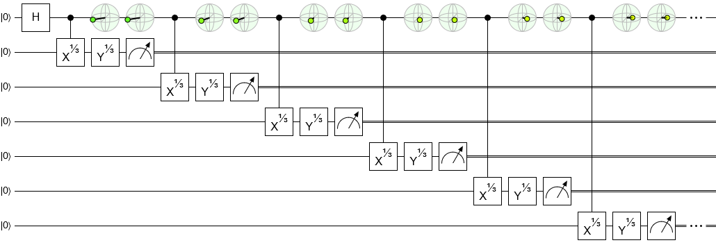
In these circuits, we have a qubit $A$ that starts in the state $\ket 0 + \ket 1$. Then we keep introducing fresh work qubits in the $\ket 0$ state, performing a small rotation controlled by $A$, and measuring the result:
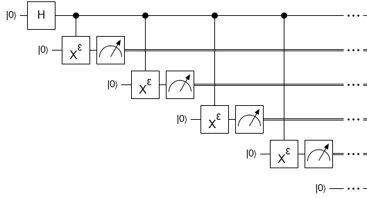
We use the measurement results to infer the state of $A$.
Surprisingly, this process plays out in qualitatively different ways depending on how you go about measuring.
Z axis
Let's start by just measuring in the computational basis, i.e. along the Z axis, as shown in the previous diagram. For flavor, we also imagine our quantum computer is setup so that any On measurement will produce an audible CLICK!.
We run the circuit. What happens?
The qubit $A$ starts in a superposition of On and Off, and that continues to be true for as long as you wait without hearing a click. But the conditional rotation creates an asymmetry between the $A$-is-Off case and the $A$-is-On case: if $A$ is Off, the conditional rotation doesn't happen. Without any rotation, the work qubit would stay Off and so the measurement result would also have to be Off. But if $A$ is On (or partially On) then, every once in awhile... CLICK! and now you know for sure that $A$ is guaranteed 100% On.
In other words, when our measurements keep happening along the Z axis, $A$ behaves like it has a half-life. We can explore this behavior in Quirk by displaying some measurement chances and conditional states:
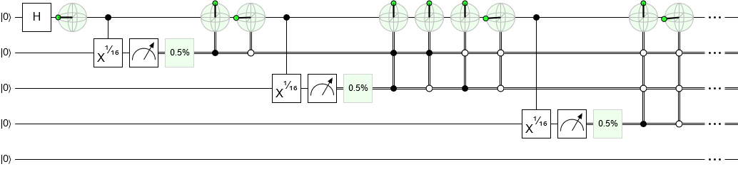
Notice how anytime a state indicator has a black "is On" control, the state is straight up (i.e. $\ket 1$), whereas the only-white-control "all Off" cases are essentially identically to the starting state. Also notice the chance-of-On staying pretty consistent. This circuit's measurements really do imply that $A$ is behaving as if its state has a half-life.
Other axis
Now lets try measuring along a different axis, by rotating the qubit a bit before the computational-basis measurement. When we do that, we see very different conditional states:
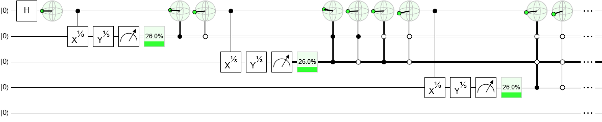
Instead of jumping to 'all on all the time' as soon as any measurement returns On, $A$ is only being perturbed a little bit by each outcome. (I had to make the conditional rotations a big stronger for it to be visible.)
If you analyze the behavior more closely, as I did in 'Eve's quantum clone computer', you find that the qubit is actually performing a random walk! Instead of waiting for a solitary click that tells you everything, you'll be hearing a stream of CLI-CLI-CLICK! CLI-CLICK! CLICK! ... CLICK! CLI-CLI-CLI-CLI-CLICK! where each click, or pause, tells you the direction of a small step the qubit took.
Interpretation
Clearly the measurement we choose to make changes the experience quite drastically. In one case we're patiently waiting for a single click that reveals all. In the other case, we're hearing a stream of clicks that together slowly build up to the full story. But what does this all mean? And is it useful?
The authors end their video with the following claim:
"This gives us a way to control the atom by the way that we look at the light."
That's actually not quite right.
Up until now, I've been showing conditional states in the circuit diagrams. But what does the qubit's unconditional state, i.e. what we can expect before even starting the experiment, look like?
Well, when measuring along the Z axis, the qubit kinda rotates slowly while decaying towards the center:
And, when measuring along another axis, the qubit... kinda rotates slowly while decaying towards the center...:
The above diagrams show that the qubit evolves in the same way, regardless of which measurements we plan to make. This demonstrates that changing the axis doesn't give us any control. (Though that was obvious from the start, since otherwise we could easily violate the no-communication theorem.)
What's actually happening during these experiments is that we're learning different information about the qubit as we go. Although the unconditional expected-ahead-of-time states don't depend on the measurement choices, the conditional informed-by-measurement states differ by quite a lot. We're not deciding what happens, but we are finding out what happened.
So the authors are wrong when they say we've found a way to control the atom by looking at the light differently. A corrected quote would be... "This gives us a way to find out if the atom is in the state we want by the way that we look at the light". Which... sounds quite a lot more mundane, doesn't it?
Still, it's very interesting that the experience changes so much when measuring different axes.
Ultimately, I think that the phenomena described by the paper is just an interesting example of how you learn different things by measuring different things. There's no control, at least not in the literal sense of the word.
(That being said, I feel uncomfortable bluntly leaving things at "there's no control". It has the wrong connotations, and probably some people will disagree about the shades of meaning. The thing we are doing would require control if this was a classical system. This is yet another example of entanglement riding the line between "I can predict that!" and "I can control that!" in a way that's hard to summarize.)
Summary
How you measure entangled information about a qubit qualitatively changes the feel of the inference process. Sometimes it behaves like spontaneous decay, other times like a random walk.
Despite the surprisingly different behaviors, we're not actually controlling the qubit. We're just revealing things about it at different rates.
Comments
Does a similar circuit represent the Quantum Zeno effect?
I know you had an earlier post about Zeno but it didn't have a circuit diagram in it. My guess is that the Qbit should have a fixed initial state and then small rotations applied along the top line, but that the presence of the conditional gates may help to preserve the Qbit in its original state?
Yes, it's a similar circuit. The main difference is that, in the Zeno effect, the small rotation is applied *to* the qubit-of-interest. Here the qubit-of-interest is controlling the small rotation. Also the Zeno effect involves constantly directly measuring the qubit-of-interest, whereas here we're only measuring related information.
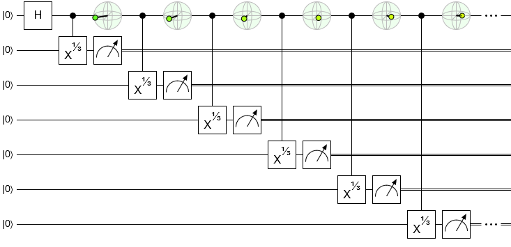
Here's a mock Zeno circuit (normally eight X^(1/8) gates would do a full NOT, but due to the intermediate CNOTs the qubit stays mostly off; the effect gets stronger with smaller rotations)
Ah, that's brilliant! I'd tried a similar circuit, but I had the control gates upside down (which fails to have any effect at all).
(By the way, the link is a bit hard to copy/paste from the comment box - I had to use developer tools to get access to the full string)
We’re delighted that you have taken an interest in our paper, and have taken the time to think it through. We certainly agree that the unconditional dynamics of decay will be the same despite how one detects the emission, and it would make no sense if that was the case. So the ‘control’ that we have over the qubit is indeed conditional. For example, if we initialize the qubit in a state along X and perform homodyne measurements of the emission, each decay trajectory will be different and some of these trajectories will result in the qubit moving toward its excited state. So if we can use the information we have collected we can effectively control the qubit to move into its excited state. Of course, this protocol does not work every time, about half the time it ends up in its ground state (so it is an uncontrolled control). Is this useful? Absolutely. In the paper, we use this type of evolution to herald different initial states that we want to study, something that could have been achieved by a complicated sequence of pulses, but instead we can allow the random quantum evolution to herald the state.
Again, this sounds like selective information, but it is in fact much deeper than that. When the qubit decays it becomes entangled with the electromagnetic field which exhibits quantum fluctuations. These fluctuations lead to the random conditional evolution of the qubit. Let’s describe the field in terms of the quadratures: a^dagger e^{i phi} + a e^{-iphi}, for phi=0 the field is coupled to the X dipole of the qubit, and for phi = pi/2 it is coupled to the Y dipole. (i.e. if I measure the field quadrature along phi=0 it gives me information about the random walk the qubit takes along the X-Z plane of the Bloch sphere, and if I measure along phi=pi/2 I get information about evolution in the Y-Z plane. So by measuring both quadratures, I would get random evolution over the whole Bloch Sphere (as was done in this very nice paper: Observing quantum state diffusion by heterodyne detection of fluorescence. Phys. Rev. X 6, 011002 (2016) )
Okay, but when we measure a specific quadrature, we actually squeeze the fluctuations of the electromagnetic field, effectively erasing the fluctuations in the phi = pi/2 quadrature, and amplifying the fluctuations in the phi=0 quadrature. In this case, the evolution of the qubit is restricted to the X-Z plane, not because we have ignored the information about diffusion in the Y-Z plane, but because we have erased that information. If our quantum efficiency was perfect, then we would maintain a perfectly pure state of the qubit. So the random walk is “controlled” in the sense that it is confined to a specific great circle of evolution, but it uncontrolled in that the evolution is still random. At the core, this is because there is entanglement between the qubit and the field, so the “control” aspect takes on similarities to a violation of Bell’s inequality. This is called "EPR steering”.
Now, I should admit that we don’t have high enough quantum efficiency to prove that we can steer the state, but this is something that we’re working on and I’ll let you know when we get there.
Thank you for commenting.
I do feel a bit bad about not explaining the lack of control more fully in the post. The content happened to overlap with a future planned post about EPR steering where I was going to go over it in more detail. (I assume EPR steering is not what you were referring to when you said 'steer the state'.)
Fair warning though: don't put too much effort into controlling the state in this way. Suppose the default sequence of axis choices succeeds at creating some desired state 10% of the time after 100 step and you come up with a better sequence that succeeds 11% of the time after 100 steps. You then pass these states along to some consumer who uses them to do something observable that succeeds more often when the qubits are in the desired state. So if you used the 10% process then the task might succeed 1% of the time, but with the 11% process the task would succeed 2% of the time.
Congratulations, you just created an FTL communication mechanism!
Alice produces a qubit and sends it to Bob, but she keeps the qubits she needs to perform the measurement sequence coherent. She repeats this many times. Later, Alice receives a message to send to Bob. Using an error correcting code, she encodes the message into the choice of using the 10%-success process or the 11%-success process. Bob receives the information by performing the task Y and tracking whether or not it succeeds (1% of the time for Off, 2% of he time for On). Although this communication channel is extremely noisy, it doesn't require any interaction between Alice and Bob except for the initial sharing of qubits.
So we can conclude, in full generality, that there's no way to improve any measurable outcome of any task by just using a clever sequence of measurements in this situation. It violates the no-communication theorem.
Of course if you *use* the measurement results, then you can control the qubit. Suppose you want qubits either in the state cos(t) |0> + sin(t) |1> for t = pi-0.1 or t=pi+0.1 but no other t. You want to feed the pi-0.1 qubits to one experiment, and the pi+0.1 qubits to another. It would be silly to use the "full decay" measurement, since both outcomes are bad. The "random walk" measurement on the other hand would do pretty well. But this is all based on the fact that you feed the measurements back into what happens to the qubit. The control doesn't come from just the measurement results, it comes from doing things to the qubit (based on the measurement results).
