

This series of posts began with the discovery a mistake, and an attempt to fix the problem. It ends with an insight into and improvement upon the original result.
Part 1: (this post) Resynthesizing the circuits
Part 2: Reconceptualizing the distillation
Part 3: Rebraiding the factory
Noticing a mistake
When I read papers describing quantum circuits, I like to test them out in my drag-and-drop quantum circuit simulator Quirk. Quirk affords fast iterative experimentation. It allows me to push the circuits around, try random ideas to make them smaller, see what makes them break, and maybe even understand what makes them work.
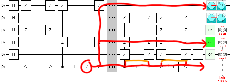
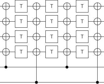
I was experimenting on circuits from the paper "Surface code implementation of block code state distillation" when I found a problem: the circuits didn't work as advertised. The mistake happens right near the beginning of the paper, in figure 1:
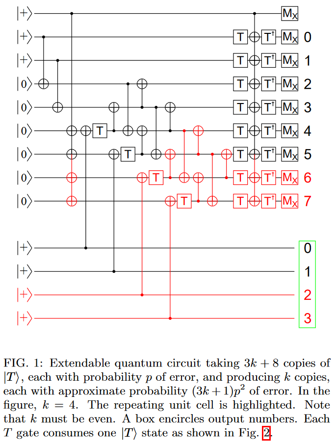
When I entered this circuit into Quirk, I wasn't able to get it to do what it was supposed to do. At first I figured this was because I simply hadn't found the correct feedback operations (annoyingly, the figure leaves out all of the classical fixup that happen after the measurements). But gradually it became clear that the problem was in the circuit itself.
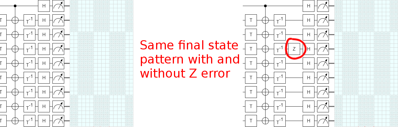
The method I used to convince myself that a mistake really is present was to realize that, since this circuit is supposed to detect single errors, inserting a Z gate next to one of the T gates should change the set of possible measurement outcomes. Otherwise the error would be undetectable. By just eyeballing the states while dragging a Z gate around (thanks, Quirk!), I was able to find several T gates where inserting a Z error doesn't change the possible measurement results. Therefore the circuit is wrong.
For example, there is no change in possible results when adding a Z gate after the third inverse T gate:
The fact that this mistake happens in figure 1 of the paper is very unfortunate, because the paper just keeps building and building on this figure. The one initial mistake poisons all of the presented details. (The k=2 case works, though!) That being said, as we will see by the end of this trilogy of posts, the high-level conclusions of the paper do survive the correction of the mistake.
I happen to work with Austin Fowler, who is the lead author of the paper, so it was very easy to bring the mistake to his attention. He acknowledged the problem, pointed me at the paper that they had intended to implement ("Magic state distillation with low overhead" by Bravi et al in 2012), and asked me to look into how hard it would be to fix the issue.
Rederiving the circuit
I wish I could say that I carefully went through the Bravi et al paper, worked through all the logic, and understood the underlying ideas. But actually what I did was skim through the paper, spot equation 3, and go "Ah! I bet that's it!":
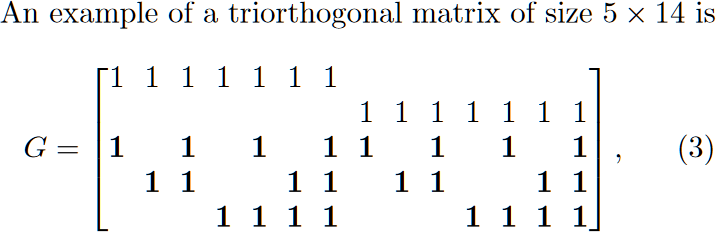
The above may not look like much, but this pattern of "several columns with different combinations of 1s" is very reminiscent of how some T state distillation works. Basically, T state distillation circuits often amount to creating several qubits in the $|+\rangle$ state and then applying T gates to various parity combinations of those qubits. I figured the matrix was saying which parities to phase (e.g. if we associate the rows with qubits $Q_0$ through $Q_4$, then the first column is saying we need to apply a T gate to $Q_0 \oplus Q_2$).
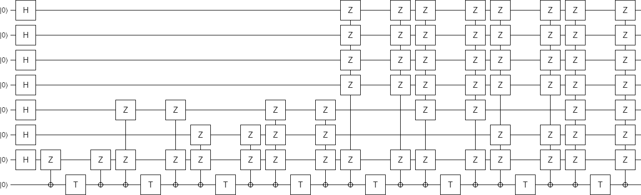
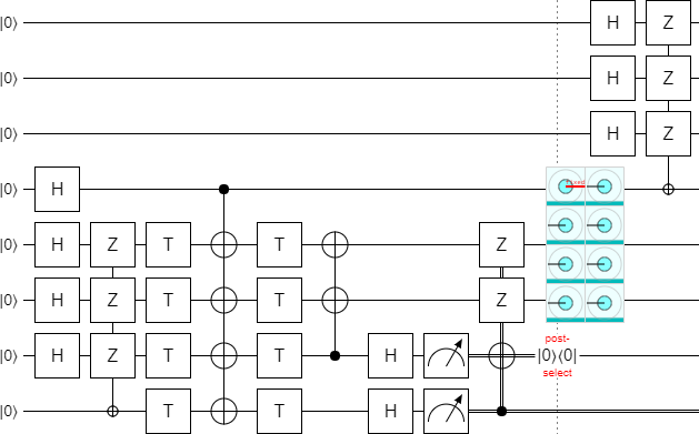
I threw together a circuit in Quirk based entirely on this guess, did some quick experimenting to figure out the classical decoding, and... it works!
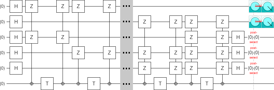
(Click the image to view the entire circuit in Quirk.)
The above circuit uses 14 T gates and produces two $|T^\dagger\rangle$ states. And if you insert exactly one Z error next to one of the T gates, the error will be caught by the post-selections. (I am assuming that the T gates are the only noisy operations, and that they can only produce Z-type errors. This is consistent with what actually happens when injecting T states in the surface code.) The circuit is producing the right amount of states with the right amount of error detection; it is correct.
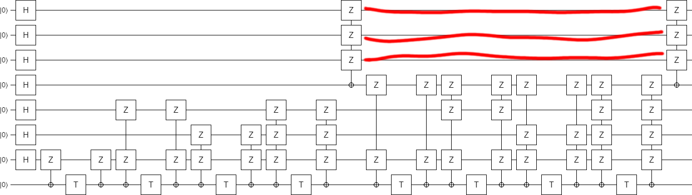
Here is one example of how a Z error will ultimately toggle one of the qubits that are measured when determining whether or not to keep the output:
So this fixed-size case works, but we're supposed to be creating an extendable construction. One with some parameter $k$ that determines how many states we make. Clearly it is necessary to carefully read the rest of the paper.
Anyways, skimming further into the paper, I spotted equations 24 and 25. They give a recipe for putting together matrices with sizes controlled by a parameter $k$:
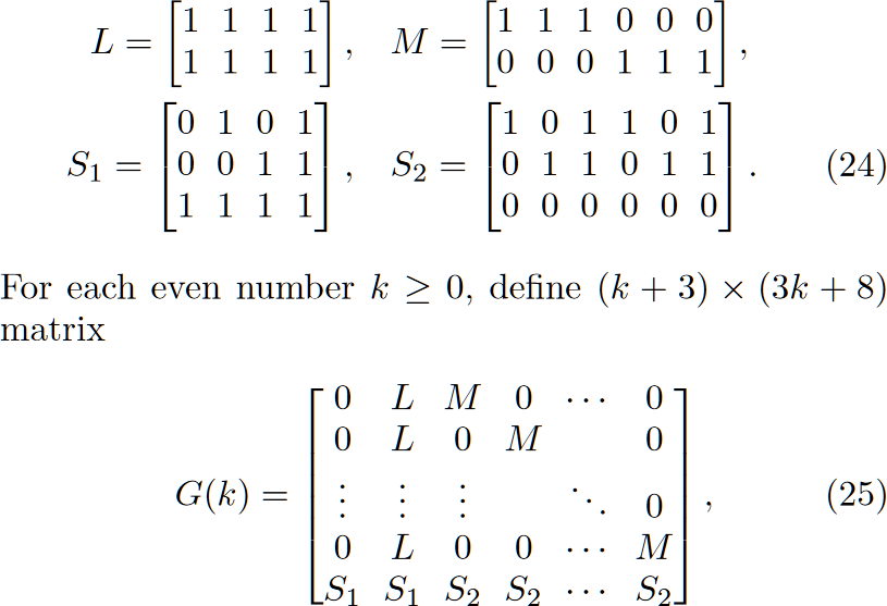
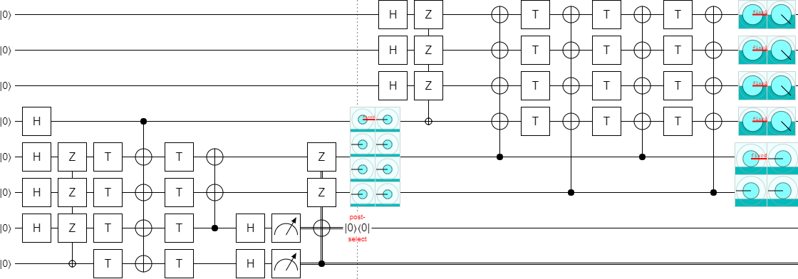
Once again, I threw together a circuit in Quirk based on my guess that the columns of the matrix were indicating which parities to phase. Getting the decoding right was a bit harder this time; some of the check qubits ended up entangled instead of separable and had to be pulled apart in order to do the post-selection properly.
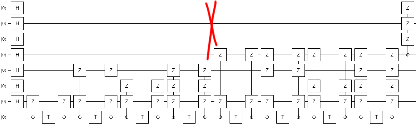
Anyways, after fixing that, I had a working k=4 circuit:
Of course, we don't want just any circuit. We want a good circuit. We've validated that the original construction works, but we still haven't validated that e.g. it can be done in constant depth. So let's do that.
Optimizing the circuit
In order to keep things simple, I am going to split the matrix defined by equations 25 and 26 (as well as the corresponding circuits that we're implementing) into two pieces and optimize each separately. This works well because the columns of the matrix split nicely into a left half (with $L$ and $S_1$ sub-matrices) and a right half (with $M$ and $S_2$ sub-matrices).
I'll focus on finite-sized cases, but all of the steps I apply will generalize to arbitrary $k$. In fact, even though the original paper only defines matrices for even $k$, the construction we end up with will also work for odd $k$!
We'll start with the left half. Specifically, this is the matrix we'll be implementing:
$$ \begin{bmatrix} M & 0 \\ 0 & M \\ S_2 & S_2 \end{bmatrix} = \begin{bmatrix} 1 & 1 & 1 & & & & & & & & & \\ & & & 1 & 1 & 1 & & & & & & \\ & & & & & & 1 & 1 & 1 & & & \\ & & & & & & & & & 1 & 1 & 1 \\ 1 & & 1 & 1 & & 1 & 1 & & 1 & 1 & & 1 \\ & 1 & 1 & & 1 & 1 & & 1 & 1 & & 1 & 1 \\ & & & & & & & & & & & \\ \end{bmatrix}$$
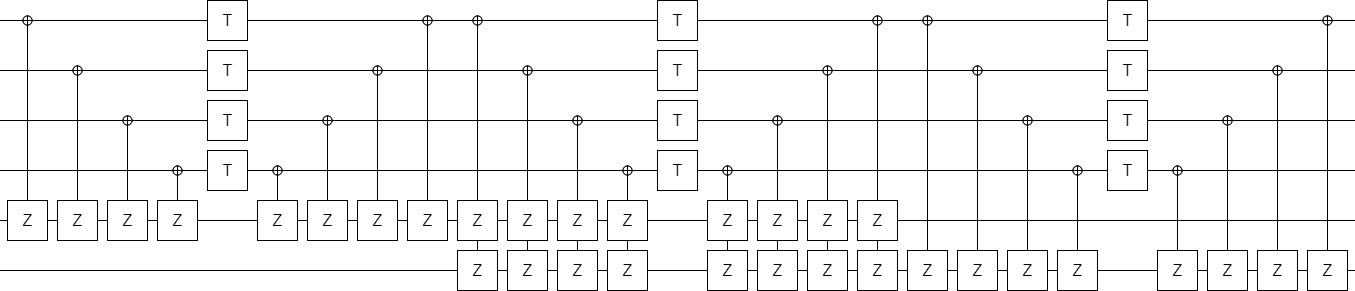
Which we can mechanically translate into this circuit:
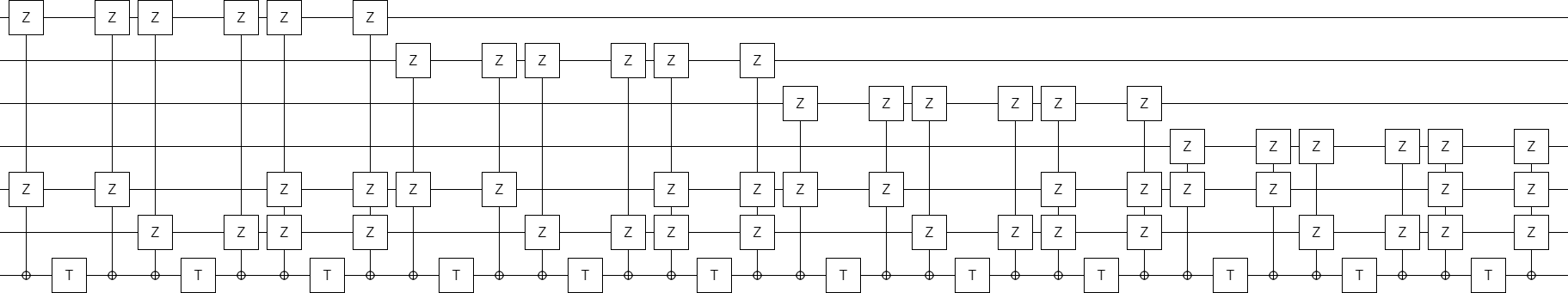
The circuits I have shown so far always use an ancilla qubit to perform the multi-qubit parity phasing operations. However, when attempting to optimize a circuit, it is usually desirable to work inline without introducing an ancilla. Instead of temporarily xoring all of the involved qubits onto a clean qubit and phasing that, we should pick one of of the involved qubits, temporarily xor the other involved qubits into the chosen qubit, and phase the chosen qubit.
Doing the phasing inline is particularly useful in this case because it makes it clear that some phasing operations can be done in parallel. In particular, the fact that the "M" sub-matrices are laid out along a diagonal suggests that inline phasing will allow them to be done in parallel.
So let's try that out. For each T gate, we need to choose which qubit to use as the inline target. In this case, we'll just always pick the topmost involved qubit. The resulting circuit looks like this:
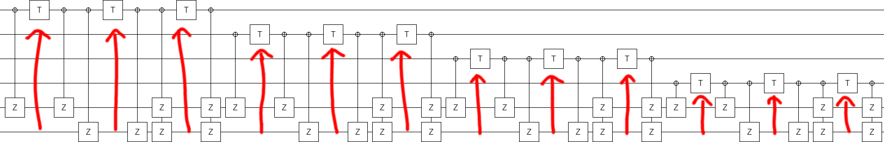
The next step to simplifying the circuit is to group the phasing operations together based which of the two bottom qubits are involved. (We can rearrange them because they all commute with each other.) First we will do all the phasing operations involving just the before-bottom qubit, then all of the phasing operations involving both bottom qubits, then all of the phasing operations involving just the bottom qubit.
Here's the circuit with the operations grouped:
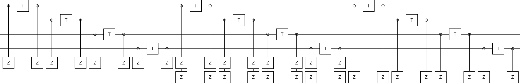
The above circuit is just begging us to do T operations at the same time. We can do this by taking advantage of the fact that the X-controlled-Z operations that are present all commute with each other (though not with the T gates). In order to move a T gate leftward into the same column as another T gate, we move the X-controlled-Z operation in its way leftward first.
Do this in the obvious way, and rearrange the X-controlled-Z operations so that they have a nice pattern, and you get this better structured circuit:
At this point it's clear that we should switch from X-axis controls and Z-axis targets to Z-axis controls and X-axis targets (i.e. use CNOT operations). Doing so folds all of the controlled operations into just a few columns, making a shallow circuit:
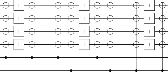
And now it's obvious that some of these controlled operations are cancelling each other out. Do the cancellations, and we're left with a nice short circuit:
If we had started with a larger value of $k$, i.e. more $M$ matrix columns, this final circuit would get taller instead of deeper (there would be $k$ copies of the top row).
Now that we've found a nice way to optimize the circuit coming from the part of the matrix involving $M$ and $S_2$, we turn our attention to optimizing the part involving $S_1$ and $L$. This will be a bit trickier to do, but don't worry we'll go through it step by step again.
This time our starting matrix is:
$$\begin{bmatrix} 0 & L \\ 0 & L \\ S_1 & S_1 \end{bmatrix} = \begin{bmatrix} & & & & 1 & 1 & 1 & 1 \\ & & & & 1 & 1 & 1 & 1 \\ & & & & 1 & 1 & 1 & 1 \\ & & & & 1 & 1 & 1 & 1 \\ & 1 & & 1 & & 1 & & 1 \\ & & 1 & 1 & & & 1 & 1 \\ 1 & 1 & 1 & 1 & 1 & 1 & 1 & 1 \\ \end{bmatrix} $$
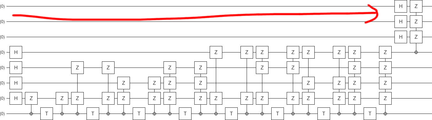
from which, keeping in mind that this part of the matrix will be at the start of our circuit, we mechanically derive a starting point:
The first thing we're going to do is try to simplify the top-right section of the circuit, because it keeps reusing the same combination of qubits again and again. Instead of depending on every one of those qubits for every phasing operation, we can xor them all into a single target qubit and then only include that one. This is the resulting circuit:
Now look carefully at the left operation we introduced in the previous step. It has an X-axis control being applied to a qubit that started as $|0\rangle$ and was then transitioned to the $|+\rangle$ state by a Hadamard operation. Applying an X-axis control to the $|+\rangle$ state is akin to applying a Z-axis control to the $|0\rangle$ state: the control is not satisfied, and all linked operations do not happen.
Therefore we can simply drop the operation:
And, suddenly, we see that the top three Hadamards can be moved all the way to the right side of the circuit. The resulting circuit has an initial part that is independent of $k$ (!), and then a single controlled operation that depends on $k$:
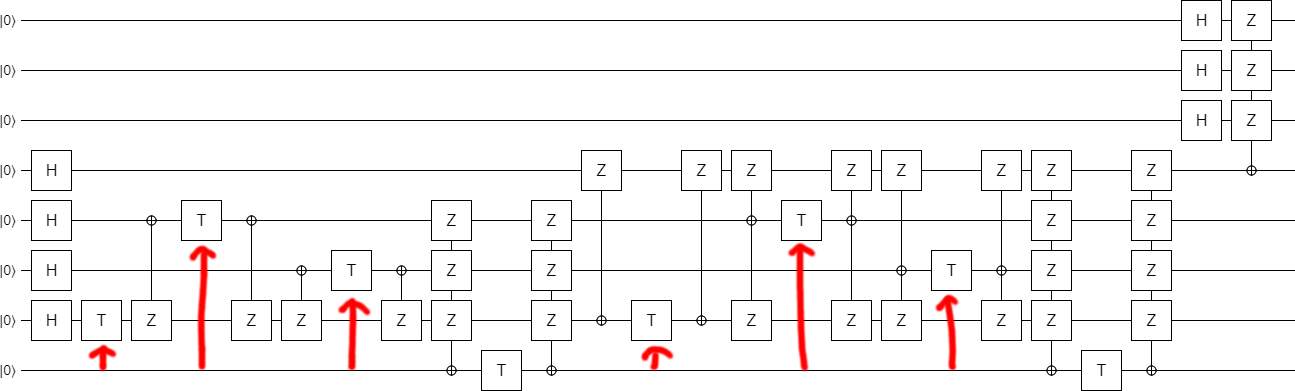
Now comes the time to switch to inline phasing. This time it's a bit harder to pick which qubits to use as the targets. And actually, because we're going to end up doing four operations at a time, one of the operations needs to continue to use an ancilla! But, with a bit of foresight, we inline the phases in the way that produces this circuit:
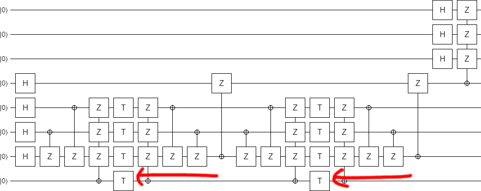
This time it's not so obvious how to move the X-controlled-Z operations out of the way, so that the T gates can be combined into columns. We start by combining the T gates that are easy to get together:
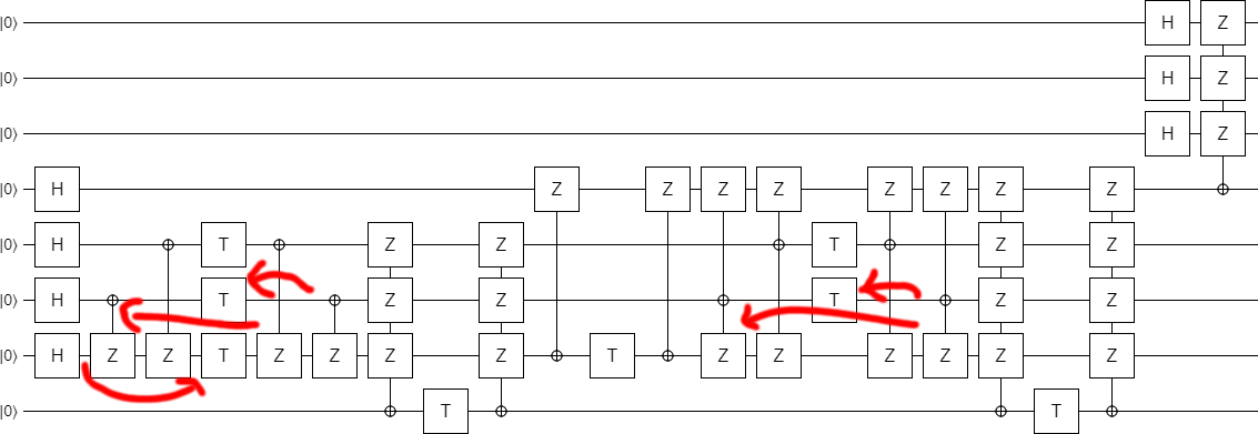
Now we do two key moves. First, we propagate the second X-controlled-Z (the one going from qubit #4 to qubit #7) rightward. This cancels out several Zs, allows a trapped T gate to be combined with the others, and makes the left part of the circuit look more like the middle part:
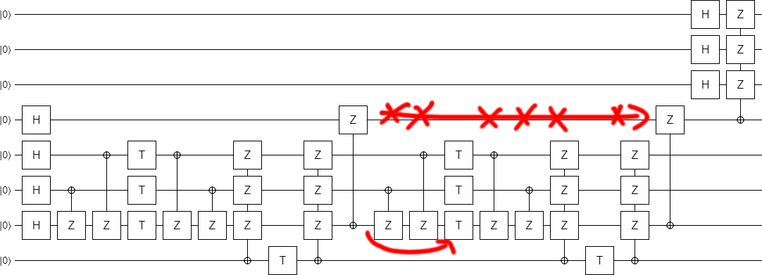
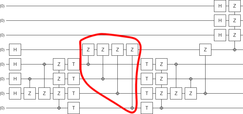
The second key move is to realize that, although the triple-Z observables do not commute with the operation to their left, they do commute with the pair of operations to their left. This allows the final T gates to be moved into place:
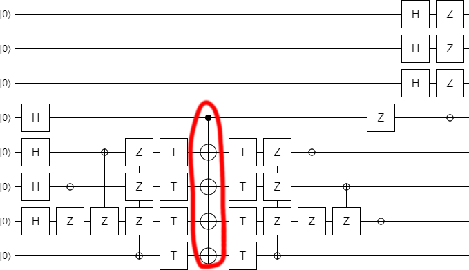
Now that the T gates are in columns, our goal is to simplify the surrounding controlled operations. If you play around with the middle section for awhile, you will find that the operations on the left can be cancelled against the operations on the right at the cost of creating extra operations targeting the fourth qubit. Basically, keep playing until you end up with this circuit:
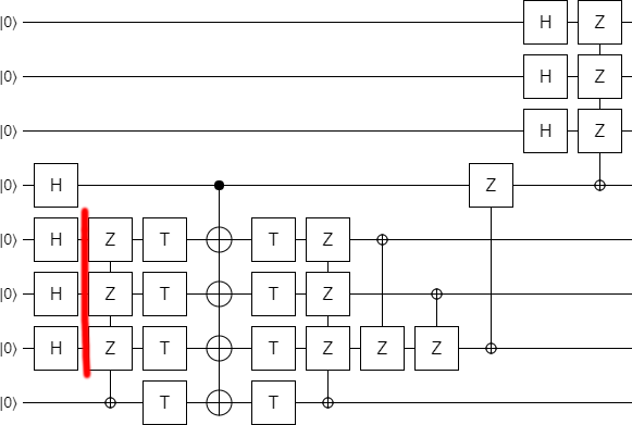
Of course, the middle is now much better represented with a single multi-target CNOT:
Next! Okay, see the first two controlled operations? They have controls that aren't satisfied. They can be dropped, producing a shorter circuit.
At this point it is clear that the bottom part of the circuit is preparing some kind of special state, which is then being expanded at the end of the circuit. What is this special state?
By adding a couple displays into the circuit, it becomes clear what's going on:
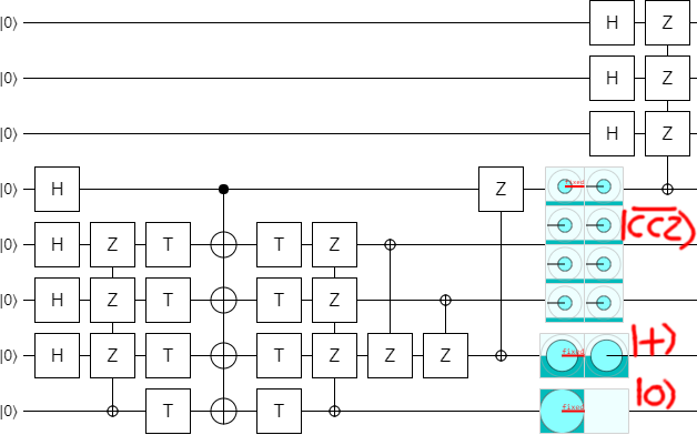
The bottom qubit ends up Off, which makes sense since we were only using it as a temporary ancilla.
The second-to-bottom qubit is ending up in the $|+\rangle$ state. That indicates that it's supposed to be a check qubit.
The next three qubits are being prepared into a superposition with equal magnitude on each of the eight possible computational basis state. However, the phases are not all the same: the $|000\rangle$ state has opposite phase to the rest. They nearly form a $|CCZ\rangle$ state (a state used to apply Toffoli gates in an error-detecting fashion), but normally the negative sign would be on the $|111\rangle$ state, not the $|000\rangle$ state. I call this slightly different state a $|\overline{CCZ}\rangle$ state (the overbar indicates that it's an "inverse" CCZ).
In the next post, I'll talk more about the significance of this $|\overline{CCZ}\rangle$ state and how recognizing it allowed me to understand in a simple way what the block code is actually doing. For now, let's move on with optimizing the circuit.
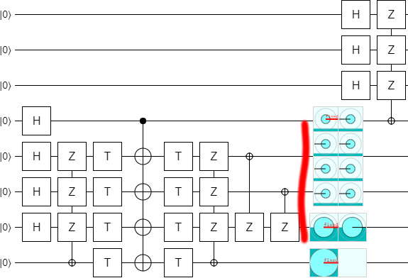
Our next optimization is an easy one, once you spot it. The last operation on the second-to-bottom qubit, the one that ends up in a $|+\rangle$ state, is a controlled operation that does nothing when said qubit is in the $|+\rangle$ state. So... drop that operation:
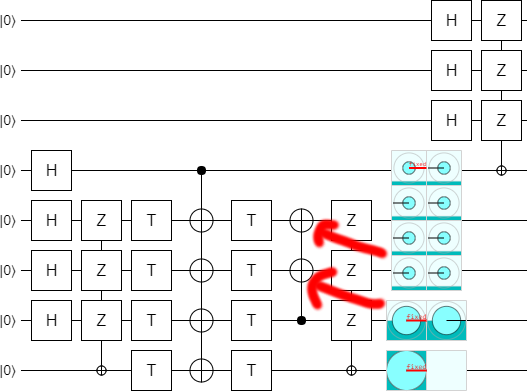
For reasons that will become obvious in the next step, we now turn the two lonely X-controlled-Zs into a multi-target CNOT, and propagate it leftward a bit:
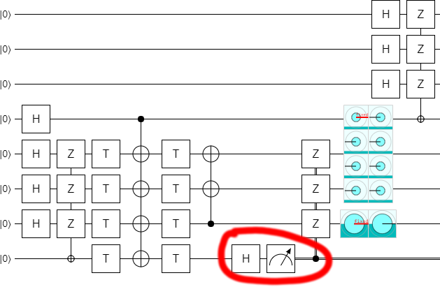
Now, notice that currently the bottom qubit is not used for anything at the end of the circuit. It is simply being uncomputed and then discarded. Therefore, instead of uncomputing it, we can get rid of it with erasure. That is to say, instead of discarding it we do a measurement that aligns with the final operations on it and then use the deferred measurement principle to propagate the measurement over that final operation. This is particularly beneficial because the classically-controlled operations we end up with in the resulting circuit are all Pauli operations, which can be propagated around the circuit very easily:
The last thing we need to do is something we probably should have done from the start: measure that the qubit that's supposed to end up in the $|+\rangle$ state does in fact end up in the $|+\rangle$ state. This gives us our optimized left-half circuit:
Now all we need to do is put this $L$ and $S_1$ piece together with the $M$ and $S_2$ piece.
Putting the pieces together
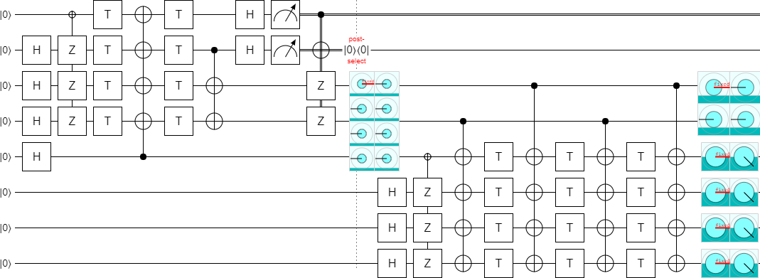
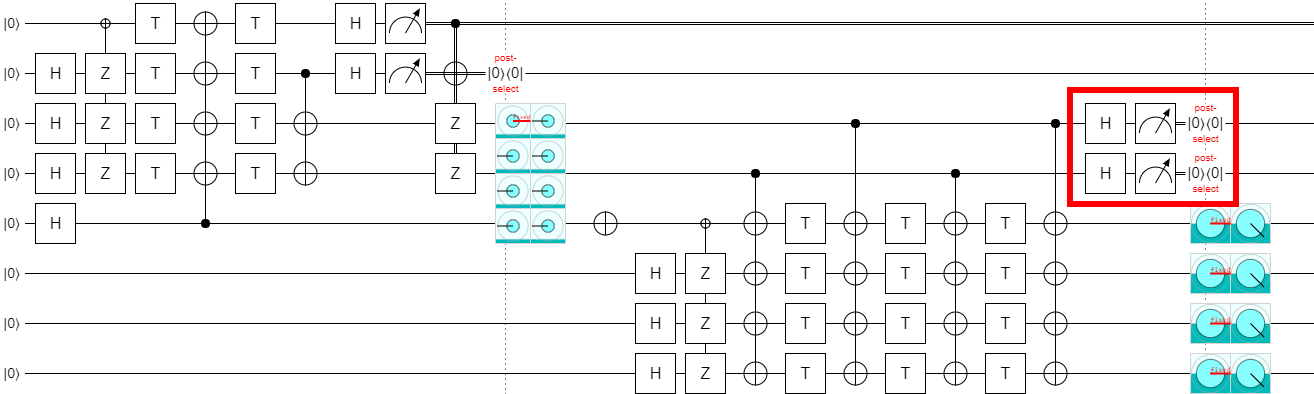
We have our separately optimized both halves of the circuit. We can combine them into a single circuit:
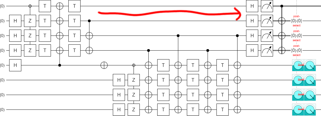
Currently, increasing the parameter $k$ would extend the circuit upward. I'd rather the circuit grow downward, so let's flip everything vertically:
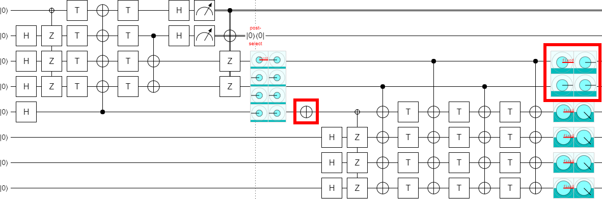
Now we need to figure out the error decoding. See how the top two used qubits on the right side are ending up in the state $|00\rangle - |01\rangle - |10\rangle - |11\rangle$? We don't want that. We want a separable state.
One way we could fix this is to apply a CZ to the two qubits, separating them into $|-\rangle$ states. But solving the problem in that way will lead us down a bad path. (Trust me, I tried.) Instead of doing that, all we need to do is insert a NOT gate... at the right place.
I should point out that I certainly wouldn't expect inserting a NOT gate to do anything useful here. The only reason I know it works is because Quirk makes it quick and easy to tweak the circuit and see how the output changes. As a result, I'm always deleting gates, adding gates, and dragging gates around just to see if they have some useful effect. It sounds completely dumb, but it pays off all the time and right here right now we have a particularly good example of that. In fact, the most serendipitous consequence of this change will only appear after several more steps.
For now, let's separate the outputs by inserting the magic NOT gate:
Now that the outputs are separated, we can post-select on them to detect errors:
And we might as well do all the measurements and post-selection in the same place:
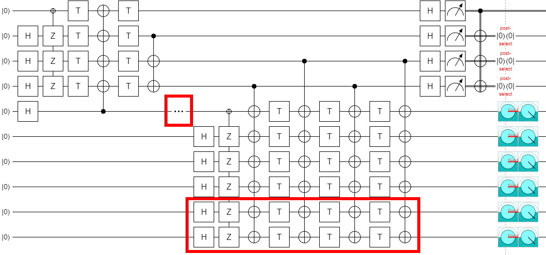
Which brings us back to that NOT gate. It turns out that, when you extend the circuit down by two steps, increasing $k$ from 4 to 6, you have to remove the NOT gate. Otherwise the output ends up in that state we didn't want, again.
In order to extend to $k=6$, delete the NOT gate:
If we increase $k$ by two more, to 8, then the NOT gate is needed again. And the pattern continues like that, where you need the NOT gate for multiples of 4 but not for numbers equal to 2 mod 4.
Now, if you remember where these circuits came from, you might also remember that they were only defined for even values of $k$. So there's no reason to expect them to generalize to odd values of $k$. But we have a very suggestive pattern here: if you go two steps, you rotate around X by an additional 180 degrees. So, that might... that might just mean...:
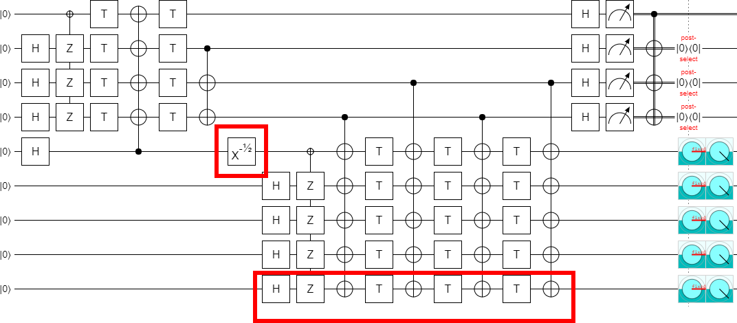
...you can make the circuit work in the odd cases by using 90 degree rotations!
Without the ability to experiment quickly in Quirk, I would never have found the location where that X gate goes. That was a key element in finding this generalization. I think this is a strong indicator that we need more tools like Quirk with a heavy focus on fast feedback and exploration... but I digress.
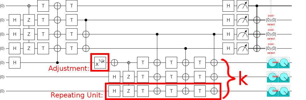
Before we finish, let's make just one more exploration-based improvement. By experimentally deleting gates, I found that one of the columns of CNOTs was redundant:
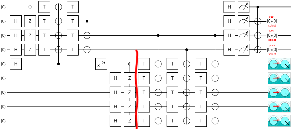
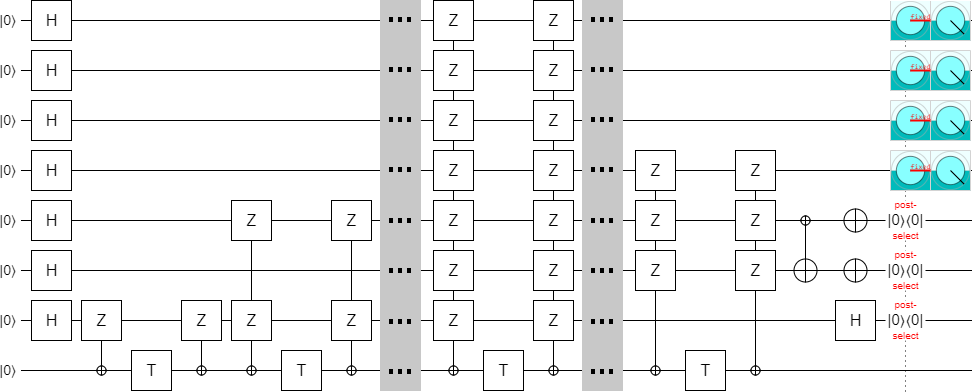
Leaving us, finally, with the final construction (at least for part 1):
This is a very nice construction, I think. Not only does it generalize the original construction so that it works for odd values, it also clearly demonstrates that it's possible to implement the circuit in constant depth (independent of $k$).
Note that I did confirm that the error detection actually works. If you insert exactly one Z error into the circuit, anywhere next to a T gate, the post-selection will detect the error and discard the state. Errors on the left side trigger the top-most post-selection, while errors on the right side trigger the other post-selections. This is pretty easy to confirm for yourself by tracing out how each Z propagates through the circuit and into the error-detecting measurements.
To be continued
Recall from the intro that this whole thing started because I discovered a mistake in a paper. The circuit construction I showed in this post fixes that initial mistake, but that doesn't mean we're done. The mistake poisoned the rest of the figures in the paper; we also need to fix those. For example, we need to translate the circuit diagram into surface code braiding diagrams.
But that's only going to happen in part 3. We're going to take a slight detour first. In part 2, I'll explain what this block code is actually doing and use that knowledge to reduce the T count of the circuit.
